Chan & Raffa 2017
Excerpt from published methods
A three-step cleaning process was used to identify outlier weights recorded in the EHR. The first step was to exclude 70,636 (0.27%) weights in the EHR with values less than 22.7 kg (50 lbs) or greater than 340.2 kg (750 lbs), as these extreme values are implausible. The second step was to calculate each Veteran’s BMI using the average height, in order to identify the 45,318 weights that were similarly implausible (defined as a BMI ≤10 or BMI ≥100) for exclusion. Then, for the third step, each Veteran’s mean weight and standard deviation were determined from the remaining weights available. Weights in the EHR that were greater than 3 standard deviations from the mean, an additional 162,349 weights, were excluded. Overall, following the three-step cleaning procedure, a total of 278,303 (1.05%) weights were excluded from the analysis leaving 26,263,946 weights available for inclusion.
Translation in pseudocode
DEFINE time t_ij for person i IN 1:I, j weights IN 1:J
FOR i IN 1:I
  FOR j IN 1:J
    IF (weight_ij < 50 lbs. OR weight_ij > 750 lbs.)
        weight_ij := NA
  END
  MEAN_i := MEAN({weight_i}_j)
  SD_i := SD({weight_i}_j)
  FOR j IN 1:J
    IF (weight_ij > MEAN_i +/- 3 * SD_i)
      weight_ij := NA
  END
END
-----------------------------------------------------
BMI := (weight_j (kg) / height (m)) ^ 2
IF (BMI <= 10 OR BMI >= 100)
    BMI := NA
Algorithm in R Code
#' @title Chan 2017 Measurment Cleaning Algorithm
#' @param DF object of class `data.frame`, containing `id` and `measures`
#' @param id string corresponding to the name of the column of patient identifiers in `DF`
#' @param measures string corresponding to the name of the column of measurements in `DF`
#' @param tmeasures string corresponding to the name of the column of measurement collection dates or times in `DF`. If `tmeasures` is a date object, there may be more than one weight on the same day, if it precise datetime object, there may not be more than one weight on the same day
#' @param outliers object of type `list` with numeric inputs corresponding to the upper and lower bound for each time entry. Default is `list(LB = 50, UB = 750)`
#' @param SDthreshold numeric scalar to be multiplied by the `SDMeasures` per `id`. E.g., from Chan 2017, "...weights greater than 3 standard deviations above the mean..." implies `SDthreshold`= 3
Chan2017.f <- function(DF,
                       id,
                       measures,
                       tmeasures,
                       outliers = list(LB = 50, UB = 750),
                       SDthreshold = 3) {

  if (!require(dplyr))      install.packages("dplyr")
  if (!require(data.table)) install.packages("data.table")

  tryCatch(
    if (!is.numeric(DF[[measures]])) {
      stop(
        print("measure data must be a numeric vector")
      )
    }
  )

  tryCatch(
    if (!is.list(outliers)) {
      stop(
        print("outliers must be placed into a list object")
      )
    }
  )

  # convert to data.table
  DT <- data.table::as.data.table(DF)
  setkeyv(DT, id)

  # Step 1: Set outliers to NA
  DT[,
     measures_aug_ := ifelse(get(measures) < outliers[[1]]
                             | get(measures) > outliers[[2]],
                             NA,
                             get(measures))
     ]

  # calc mean of measures per group
  DT[, meanMeasures := mean(measures_aug_, na.rm = TRUE), by = id]
  # calc SD of weight per group
  DT[, SDMeasures := sd(measures_aug_,   na.rm = TRUE), by = id]

  # calc UB and LB
  DT[, LB := meanMeasures - (SDthreshold * SDMeasures)]
  DT[, UB := meanMeasures + (SDthreshold * SDMeasures)]

  # Step 2: outliers bounded by SDthreshold
  DT[,
     measures_aug_ := ifelse(measures_aug_ < LB | measures_aug_ > UB,
                             NA,
                             measures_aug_)
     ]

  DT <- DT %>% select(-UB, -LB)
  DT
}
Algorithm in SAS Code
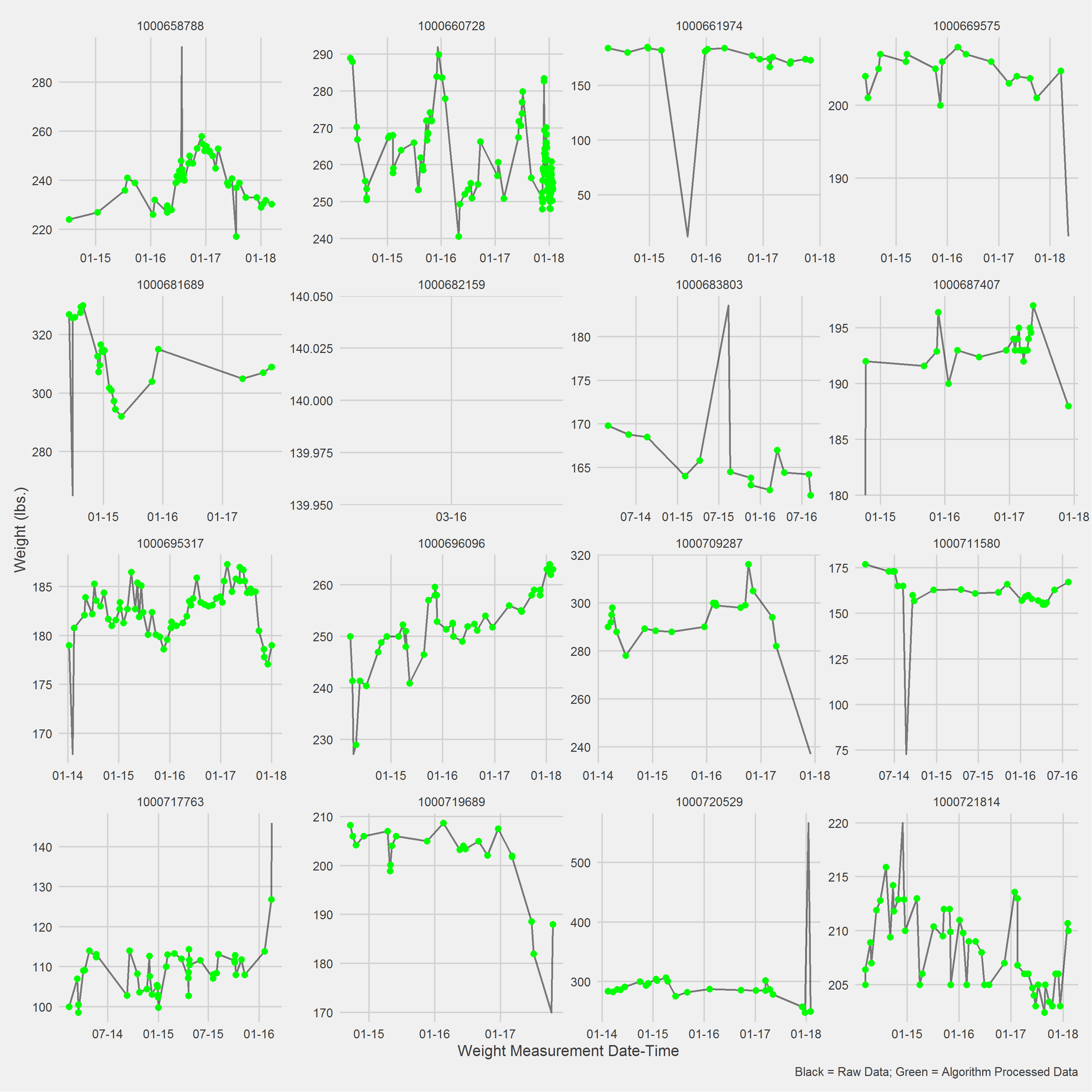
Example in R
Displaying a Vignette of 16 selected patients with at least 1 weight observation removed.
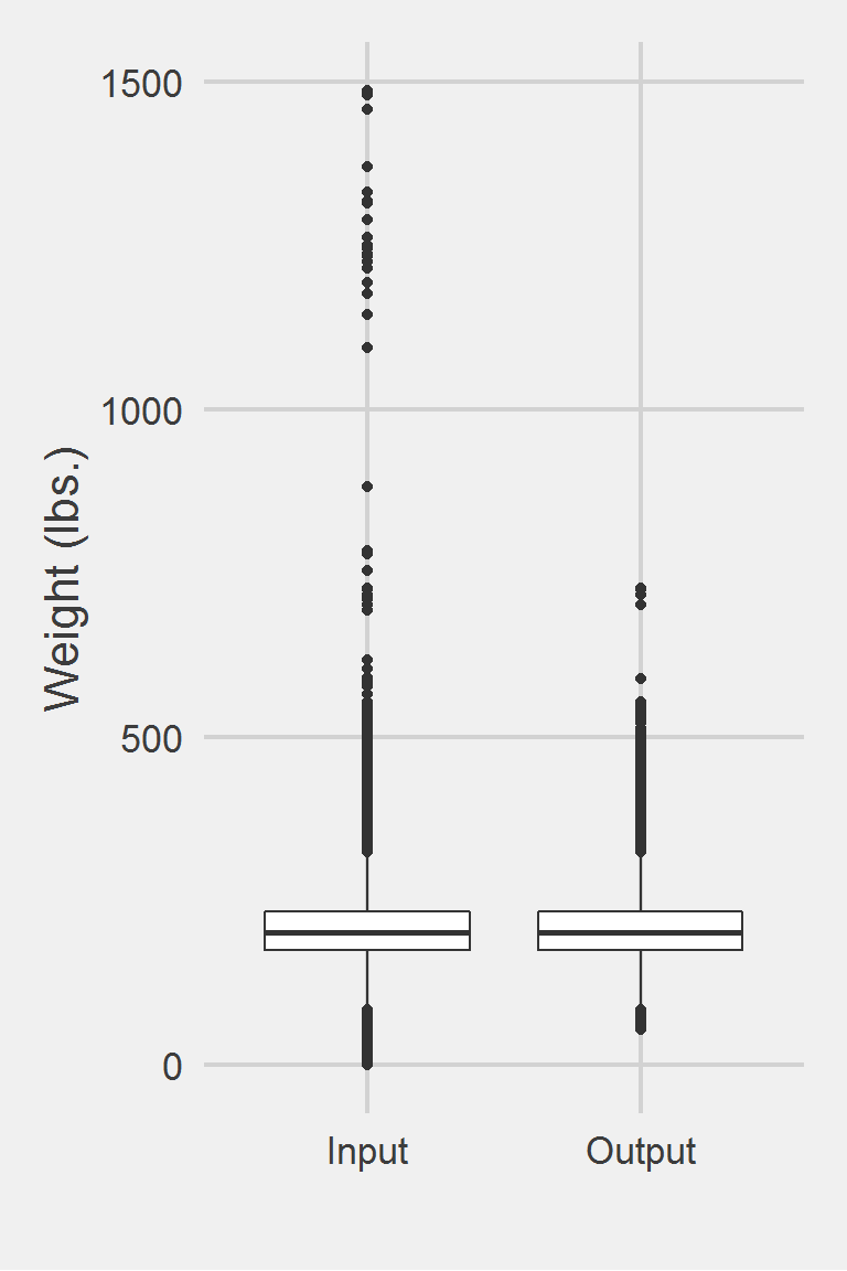
Distribution of Weight Measurements between Raw and Algorithm-Processed Values
 Descriptive statistics by group
group: Input
   vars       n   mean   sd median trimmed   mad min    max  range skew
X1    1 1175995 207.82 48.6  202.3  204.62 44.18   0 1486.2 1486.2 0.98
   kurtosis   se
X1      5.6 0.04
------------------------------------------------------------
group: Output
   vars       n   mean    sd median trimmed   mad min   max range skew kurtosis
X1    1 1170114 207.86 48.27  202.4  204.66 44.18  54 727.5 673.5 0.81     1.45
     se
X1 0.04
Left boxplot is raw data from 2016, PCP visit subjects while the right boxplot describes the output from running Chan2017.f()