Overall Sample Comparison

weightSamples <- weightSamples %>%
  left_join(
    ModeOfHeight %>%
      select(-freq),
    by = "PatientICN"
  ) %>%
  mutate(BMI = 703 * Weight / (Height ^ 2)) %>%
  select(-Height) %>%
  distinct(PatientICN, WeightDate, Weight, .keep_all = TRUE)

weight.ls <- vector("list", 2)
weight.ls[[1]] <- weightSamples %>%
  filter(SampleYear == "2008" & !is.na(Weight))
weight.ls[[2]] <- weightSamples %>%
  filter(SampleYear == "2016" & !is.na(Weight))

lsnames <- c("PCP2008", "PCP2016")
names(weight.ls) <- lsnames

rm(weightSamples)

Aggregating over each year, the mean and standard deviation of weight is 205.2 (48.2).

mean	min	max
12.05	1	1525

On average, each veteran has 12 weights recorded over a 4-year collection period, and at least 1 person has 1,525 measurements collected. 5291 veterans have only 1 weight measurement recorded.

SampleYear	mean	sd
2008	202.71	47.65
2016	207.82	48.60

Between 2008 and 2016, the average weight increased by about 5 lbs. (202.7 to 207.8), and a 1 point increase in standard deviation.

SampleYear	mean	min	max
2008	12.09	1	1457
2016	11.88	1	1525

The number of weights recorded does not differ between the 2008 and 2016 cohorts, the average and range of each being nearly identical to the overall distribution.

By Algorithm

raw <- bind_rows(weight.ls, .id = "Cohort") %>%
  select(Cohort, PatientICN, Weight, Sta3n)

#---- apply Janney et al. 2016 ----#

Janney2016.ls <- lapply(
  weight.ls,
  FUN = function(x){
    Janney2016.f(
      DF = x,
      id = "PatientICN",
      measures = "Weight",
      tmeasures = "WeightDateTime",
      startPoint = "VisitDateTime"
    )
  }
)

# post-process for joining with other algorithm output
Janney2016.df <- bind_rows(Janney2016.ls, .id = "Cohort") %>%
  select(Cohort, PatientICN, Weight_OR, Sta3n) %>%
  rename(Weight = Weight_OR) %>%
  na.omit()

Janney2016.PCP16 <- Janney2016.ls[["PCP2016"]]
rm(Janney2016.ls)

#---- apply Littman et al. 2012 ----#

Littman2012.ls <- lapply(
  weight.ls,
  FUN = function(x) {
    Littman2012.f(
      DF = x,
      id = "PatientICN",
      measures = "Weight",
      tmeasures = "WeightDateTime"
    )
  }
)

Littman2012.df <- bind_rows(Littman2012.ls, .id = "Cohort") %>%
  select(Cohort, PatientICN, OutputMeasurement, Sta3n) %>%
  rename(Weight = OutputMeasurement) %>%
  na.omit()

Littman2012.PCP16 <- Littman2012.ls[["PCP2016"]]
rm(Littman2012.ls)

#---- Coerce Maciejewski et al. 2016 to a workable format ----#

maciejewski.df <- maciejewski %>%
  filter(IO == "Output") %>%
  mutate(
    Cohort = paste0("PCP", SampleYear),
    PatientICN = as.character(PatientICN)
  ) %>%
  left_join(
    raw %>%
      distinct(PatientICN, Sta3n),
    by = "PatientICN"
  )

Maciejewski2016.df <- maciejewski.df %>%
  select(Cohort, PatientICN, Weight, Sta3n) %>%
  na.omit()

Maciejewski2016.PCP16 <- maciejewski.df %>% filter(Cohort == "PCP2016")
rm(maciejewski.df)

#---- Apply Breland et al. 2017 ----#

Breland2017.ls <- lapply(
  weight.ls,
  FUN = function(x) {
    Breland2017.f(
      DF = x,
      id = "PatientICN",
      measures = "Weight",
      tmeasures = "WeightDateTime"
    )
  }
)

Breland2017.df <- bind_rows(Breland2017.ls, .id = "Cohort") %>%
  select(Cohort, PatientICN, measures_aug_, Sta3n) %>%
  rename(Weight = measures_aug_) %>%
  na.omit()

Breland2017.PCP16 <- Breland2017.ls[["PCP2016"]]
rm(Breland2017.ls)

#---- Apply Maguen et al. 2013 ----#

Maguen2013.ls <- lapply(
  weight.ls,
  FUN = function(x) {
    Maguen2013.f(
      DF = x,
      id = "PatientICN",
      measures = "Weight",
      tmeasures = "WeightDateTime",
      variables = c("AgeAtVisit", "Gender")
    )
  }
)

Maguen2013.df <- bind_rows(Maguen2013.ls, .id = "Cohort") %>%
  select(Cohort, PatientICN, Output, Sta3n) %>%
  rename(Weight = Output) %>%
  na.omit()

Maguen2013.PCP16 <- Maguen2013.ls[["PCP2016"]]
rm(Maguen2013.ls)

#---- Apply Goodrich 2016 ----#

Goodrich2016.ls <- lapply(
  weight.ls,
  FUN = function(x) {
    Goodrich2016.f(
      DF = x,
      id = "PatientICN",
      measures = "Weight",
      tmeasures = "WeightDateTime",
      startPoint = "VisitDateTime"
    )
  }
)

Goodrich2016.df <- bind_rows(Goodrich2016.ls, .id = "Cohort") %>%
  select(Cohort, PatientICN, output, Sta3n) %>%
  rename(Weight = output) %>%
  na.omit()

Goodrich2016.PCP16 <- Goodrich2016.ls[["PCP2016"]]
rm(Goodrich2016.ls)

#---- Apply Chan & Raffa 2017 ----#

Chan2017.ls <- lapply(
  weight.ls,
  FUN = function(x) {
    Chan2017.f(
      DF = x,
      id = "PatientICN",
      measures = "Weight",
      tmeasures = "WeightDateTime"
    )
  }
)

Chan2017.df <- bind_rows(Chan2017.ls, .id = "Cohort") %>%
  select(Cohort, PatientICN, measures_aug_, Sta3n) %>%
  rename(Weight = measures_aug_) %>%
  na.omit()

Chan2017.PCP16 <- Chan2017.ls[["PCP2016"]]
rm(Chan2017.ls)

#---- Apply Jackson et al. 2015 ----#

Jackson2015.ls <- lapply(
  weight.ls,
  FUN = function(x) {
    Jackson2015.f(
      DF = x,
      id = "PatientICN",
      measures = "Weight",
      tmeasures = "WeightDateTime",
      startPoint = "VisitDateTime"
    )
  }
)

# re-insert Sta3n data
for (i in 1:length(Jackson2015.ls)) {
  Jackson2015.ls[[i]] <- Jackson2015.ls[[i]] %>%
    left_join(weight.ls[[i]] %>%
                distinct(PatientICN, Sta3n),
              by = "PatientICN")
}

Jackson2015.df <- bind_rows(Jackson2015.ls, .id = "Cohort") %>%
  select(Cohort, PatientICN, Sta3n, output) %>%
  rename(Weight = output) %>%
  na.omit()

Jackson2015.PCP16 <- Jackson2015.ls[["PCP2016"]]
rm(Jackson2015.ls)

#---- Apply Buta et al., 2018 ----#

Buta2018.ls <- lapply(
  weight.ls,
  FUN = function(x) {
    Buta2018.f(
      DF = x,
      id = "PatientICN",
      measures = "BMI",
      tmeasures = "WeightDateTime"
    )
  }
)

Buta2018.df <- bind_rows(Buta2018.ls, .id = "Cohort") %>%
  select(Cohort, PatientICN, Sta3n, Weight) %>%
  na.omit()

Buta2018.PCP16 <- Buta2018.ls[["PCP2016"]]
rm(Buta2018.ls)

#---- Apply Kazerooni & Lim, 2016 ----#

Kazerooni2016.ls <- lapply(
  weight.ls,
  FUN = function(x) {
    Kazerooni2016.f(
      DF = x,
      id = "PatientICN",
      measures = "Weight",
      tmeasures = "WeightDateTime",
      startPoint = "VisitDateTime"
    )
  }
)

Kazerooni2016.df <- bind_rows(Kazerooni2016.ls, .id = "Cohort") %>%
  select(Cohort, PatientICN, Sta3n, Weight) %>%
  na.omit()

Kazerooni2016.PCP16 <- Kazerooni2016.ls[["PCP2016"]]
rm(Kazerooni2016.ls)

#---- Apply Noel et al., 2012 ----#

Noel2012.ls <- lapply(
  weight.ls,
  FUN = function(x) {
    Noel2012.f(
      DF = x,
      id = "PatientICN",
      measures = "Weight",
      tmeasures = "WeightDateTime"
    )
  }
)

Noel2012.df <- bind_rows(Noel2012.ls, .id = "Cohort") %>%
  distinct(Cohort, PatientICN, Sta3n, FYQ, Qmedian) %>%
  select(-FYQ) %>%
  rename(Weight = Qmedian) %>%
  na.omit()

Noel2012.PCP16 <- Noel2012.ls[["PCP2016"]]
rm(Noel2012.ls)

#---- Apply Rosenberger et al., 2011 ----#

Rosenberger2011.ls <- lapply(
  weight.ls,
  FUN = function(x) {
    Rosenberger2011.f(
      DF = x,
      id = "PatientICN",
      tmeasures = "WeightDateTime",
      startPoint = "VisitDateTime",
      pad = 1
    )
  }
)

Rosenberger2011.df <- bind_rows(Rosenberger2011.ls, .id = "Cohort") %>%
  select(Cohort, PatientICN, Sta3n, Weight) %>%
  na.omit()

Rosenberger2011.PCP16 <- Rosenberger2011.ls[["PCP2016"]]
rm(Rosenberger2011.ls)

# stack original (raw), janney 2016, littman 2012, maciejewski 2016, 
# Breland 2017, Maguen 2013, Goodrich 2016, Chan & Raffa 2017, 
# Jackson 2015, Buta 2018, Kazerooni & Lim 2016, Noel 2012,
# and Rosenberger 2011 processed weights
  
cohort.fac <- c("PCP2008", "PCP2016")
cohort.labels <- c("PCP 2008", "PCP 2016")
algos.fac  <- c("Raw Weights",
                "Janney 2016",
                "Littman 2012",
                "Maciejewski 2016",
                "Breland 2017",
                "Maguen 2013",
                "Goodrich 2016",
                "Chan 2017",
                "Jackson 2015",
                "Buta 2018",
                "Kazerooni 2016",
                "Noel 2012",
                "Rosenberger 2011")

DF <- bind_rows(
  list(`Raw Weights`      = raw,
       `Janney 2016`      = Janney2016.df,
       `Littman 2012`     = Littman2012.df,
       `Maciejewski 2016` = Maciejewski2016.df,
       `Breland 2017`     = Breland2017.df,
       `Maguen 2013`      = Maguen2013.df,
       `Goodrich 2016`    = Goodrich2016.df,
       `Chan 2017`        = Chan2017.df,
       `Jackson 2015`     = Jackson2015.df,
       `Buta 2018`        = Buta2018.df,
       `Kazerooni 2016`   = Kazerooni2016.df,
       `Noel 2012`        = Noel2012.df,
       `Rosenberger 2011` = Rosenberger2011.df),
  .id = "Algorithm"
)

rm(
  Buta2018.df,
  Kazerooni2016.df,
  Noel2012.df,
  Rosenberger2011.df,
  Breland2017.df,
  Chan2017.df,
  Goodrich2016.df,
  Jackson2015.df,
  Janney2016.df,
  Littman2012.df,
  Maciejewski2016.df,
  Maguen2013.df,
  raw
)

DF$Cohort <- factor(DF$Cohort, levels = cohort.fac, labels = cohort.labels)
DF$Algorithm <- factor(DF$Algorithm, levels = algos.fac, labels = algos.fac)
DF$Type <- case_when(
  DF$Algorithm == "Raw Weights"                  ~ 1,
  DF$Algorithm %in% algos.fac[c(2, 7, 9, 11:13)] ~ 2,
  DF$Algorithm %in% algos.fac[c(3:6, 8, 10)]     ~ 3
)
DF$Type <- factor(DF$Type, 1:3, c("Raw", "Time-Periods", "Time-Series"))

Total weight measurements, by algorithm and cohort year.

DF %>%
  tabyl(Algorithm, Cohort) %>%
  tableStyle()

Algorithm	PCP 2008	PCP 2016
Raw Weights	1193976	1175995
Janney 2016	209591	199830
Littman 2012	1176644	1161661
Maciejewski 2016	1168701	1146995
Breland 2017	1191360	1175177
Maguen 2013	1050974	1037293
Goodrich 2016	209447	199803
Chan 2017	1186602	1170114
Jackson 2015	264829	251501
Buta 2018	1145268	1131996
Kazerooni 2016	87489	71961
Noel 2012	721118	683008
Rosenberger 2011	246594	227215

Aggregating over Year

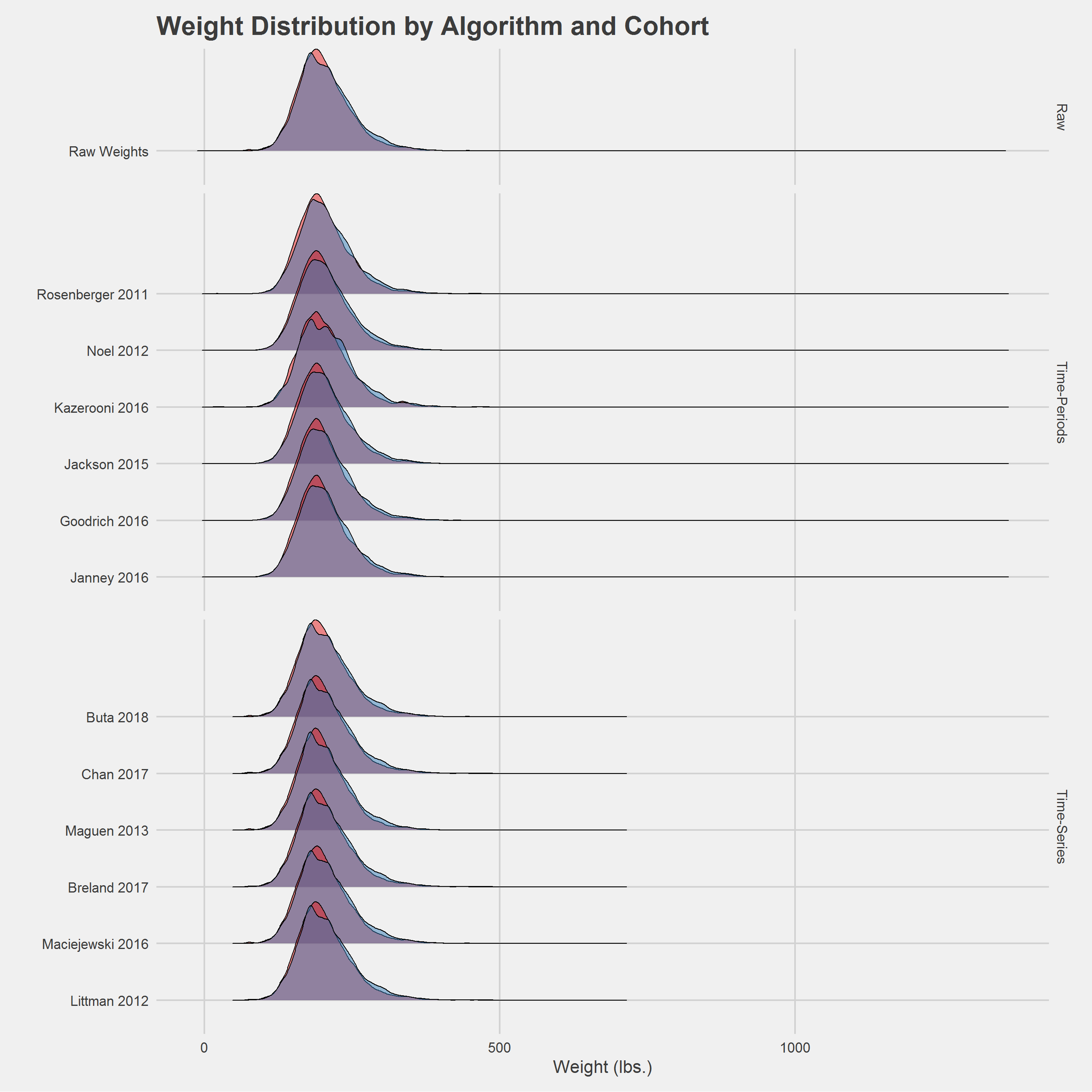
Distribution of weight measurements, by algorithm, aggregating over 2008 and 2016,

DF %>%
  filter(!is.na(Weight)) %>%
  group_by(Algorithm) %>%
  dplyr::summarise(
    weight_n = n(),
    mean     = mean(Weight),
    SD       = sd(Weight),
    median   = median(Weight),
    IQR      = IQR(Weight),
    min      = min(Weight),
    max      = max(Weight)
  ) %>%
  tableStyle()

Algorithm	weight_n	mean	SD	median	IQR	min	max
Raw Weights	2369971	205.24	48.19	199.6	58.60	0.0	2423.35
Janney 2016	409421	203.61	44.72	198.0	55.20	72.0	595.25
Littman 2012	2338305	205.43	47.31	199.9	58.60	75.0	595.00
Maciejewski 2016	2315696	205.47	47.30	200.0	58.60	53.9	632.50
Breland 2017	2366537	205.31	47.44	199.7	58.50	75.0	694.46
Maguen 2013	2088267	203.06	45.41	198.0	56.62	70.1	586.00
Goodrich 2016	409250	203.57	44.59	198.0	55.10	80.0	500.00
Chan 2017	2356716	205.31	47.47	199.7	58.50	50.0	727.50
Jackson 2015	516330	203.83	44.79	198.4	55.60	75.0	629.50
Buta 2018	2277264	205.36	47.50	199.9	58.71	60.0	571.10
Kazerooni 2016	159450	206.19	47.53	200.7	58.30	0.0	1490.00
Noel 2012	1404126	204.69	45.37	199.0	56.15	70.0	630.00
Rosenberger 2011	473809	205.14	45.73	200.0	55.96	0.0	1478.30

Number of Patients/Veterans Retained, by algorithm, aggregating over 2008 and 2016,

DF %>%
  filter(!is.na(Weight)) %>%
  group_by(Algorithm) %>%
  distinct(PatientICN) %>%
  count() %>%
  tableStyle()

Algorithm	n
Raw Weights	196625
Janney 2016	191104
Littman 2012	191323
Maciejewski 2016	196622
Breland 2017	196621
Maguen 2013	195492
Goodrich 2016	191109
Chan 2017	191327
Jackson 2015	192453
Buta 2018	179015
Kazerooni 2016	53015
Noel 2012	196622
Rosenberger 2011	131012

Number of weights retained, per person, by algorithm, aggregating over 2008 and 2016 samples,

DF %>%
  filter(!is.na(Weight)) %>%
  group_by(Algorithm, PatientICN) %>%
  count() %>%
  ungroup() %>%
  group_by(Algorithm) %>%
  summarize(
    mean   = mean(n),
    SD     = sd(n),
    min    = min(n),
    Q1     = fivenum(n)[2],
    median = median(n),
    Q3     = fivenum(n)[4],
    max    = max(n)
  ) %>%
  tableStyle()

Algorithm	mean	SD	min	Q1	median	Q3	max
Raw Weights	12.05	17.27	1	5	8	15	1525
Janney 2016	2.14	0.79	1	2	2	3	6
Littman 2012	12.22	17.15	2	5	8	15	1524
Maciejewski 2016	11.78	13.78	1	5	8	14	784
Breland 2017	12.04	17.22	1	5	8	14	1524
Maguen 2013	10.68	14.97	1	4	7	13	1516
Goodrich 2016	2.14	0.79	1	2	2	3	6
Chan 2017	12.32	17.27	2	5	8	15	1517
Jackson 2015	2.68	1.01	1	2	3	3	8
Buta 2018	12.72	17.83	2	5	9	15	1524
Kazerooni 2016	3.01	0.15	3	3	3	3	6
Noel 2012	7.14	3.76	1	4	7	10	34
Rosenberger 2011	3.62	0.55	3	3	4	4	8

By Cohort

DF %>%
  filter(!is.na(Weight)) %>%
  group_by(Algorithm, Cohort) %>%
  dplyr::summarise(
    weight_n = n(),
    mean     = mean(Weight),
    SD       = sd(Weight),
    median   = median(Weight),
    IQR      = IQR(Weight),
    min      = min(Weight),
    max      = max(Weight)
  ) %>%
  ungroup() %>%
  tableStyle()

Algorithm	Cohort	weight_n	mean	SD	median	IQR	min	max
Raw Weights	PCP 2008	1193976	202.71	47.65	197.00	57.00	0.00	2423.35
Raw Weights	PCP 2016	1175995	207.82	48.60	202.30	60.40	0.00	1486.20
Janney 2016	PCP 2008	209591	201.18	43.86	195.70	53.70	72.00	595.25
Janney 2016	PCP 2016	199830	206.15	45.46	201.00	56.70	78.40	546.00
Littman 2012	PCP 2008	1176644	202.91	46.34	197.00	56.80	75.00	595.00
Littman 2012	PCP 2016	1161661	207.97	48.14	202.60	60.00	75.20	546.00
Maciejewski 2016	PCP 2008	1168701	202.91	46.33	197.00	56.70	53.90	632.50
Maciejewski 2016	PCP 2016	1146995	208.08	48.13	202.70	60.00	62.00	546.00
Breland 2017	PCP 2008	1191360	202.81	46.49	197.00	57.00	75.00	632.50
Breland 2017	PCP 2016	1175177	207.85	48.25	202.40	60.30	75.00	694.46
Maguen 2013	PCP 2008	1050974	200.57	44.31	195.00	54.80	70.10	586.00
Maguen 2013	PCP 2016	1037293	205.58	46.37	200.70	58.28	70.30	541.10
Goodrich 2016	PCP 2008	209447	201.12	43.65	195.70	53.70	80.00	496.04
Goodrich 2016	PCP 2016	199803	206.13	45.42	201.00	56.70	80.00	500.00
Chan 2017	PCP 2008	1186602	202.79	46.53	197.00	57.00	50.00	632.50
Chan 2017	PCP 2016	1170114	207.86	48.27	202.40	60.30	54.00	727.50
Jackson 2015	PCP 2008	264829	201.48	43.96	196.00	53.70	75.00	629.50
Jackson 2015	PCP 2016	251501	206.31	45.52	201.05	56.96	75.63	553.00
Buta 2018	PCP 2008	1145268	202.84	46.57	197.00	57.00	60.50	571.10
Buta 2018	PCP 2016	1131996	207.91	48.29	202.60	60.20	60.00	540.00
Kazerooni 2016	PCP 2008	87489	203.87	47.06	198.00	56.80	0.00	1490.00
Kazerooni 2016	PCP 2016	71961	209.00	47.95	204.00	60.00	0.00	1233.70
Noel 2012	PCP 2008	721118	202.26	44.50	196.50	54.20	70.00	630.00
Noel 2012	PCP 2016	683008	207.25	46.13	202.00	57.60	70.00	588.90
Rosenberger 2011	PCP 2008	246594	202.68	45.13	197.00	54.30	0.00	1478.30
Rosenberger 2011	PCP 2016	227215	207.80	46.23	202.90	57.90	0.00	1314.50

Number of Patients/Veterans Retained

DF %>%
  filter(!is.na(Weight)) %>%
  group_by(Cohort, Algorithm) %>%
  distinct(PatientICN) %>%
  count() %>%
  ungroup() %>%
  tableStyle()

Cohort	Algorithm	n
PCP 2008	Raw Weights	98786
PCP 2008	Janney 2016	96420
PCP 2008	Littman 2012	96292
PCP 2008	Maciejewski 2016	98782
PCP 2008	Breland 2017	98782
PCP 2008	Maguen 2013	98246
PCP 2008	Goodrich 2016	96419
PCP 2008	Chan 2017	96294
PCP 2008	Jackson 2015	96984
PCP 2008	Buta 2018	89944
PCP 2008	Kazerooni 2016	29163
PCP 2008	Noel 2012	98783
PCP 2008	Rosenberger 2011	68232
PCP 2016	Raw Weights	98958
PCP 2016	Janney 2016	95742
PCP 2016	Littman 2012	96130
PCP 2016	Maciejewski 2016	98958
PCP 2016	Breland 2017	98958
PCP 2016	Maguen 2013	98352
PCP 2016	Goodrich 2016	95748
PCP 2016	Chan 2017	96132
PCP 2016	Jackson 2015	96559
PCP 2016	Buta 2018	90159
PCP 2016	Kazerooni 2016	23987
PCP 2016	Noel 2012	98958
PCP 2016	Rosenberger 2011	63405

Number of weights retained, per person, by algorithm and Cohort,

DF %>%
  filter(!is.na(Weight)) %>%
  group_by(Cohort, Algorithm, PatientICN) %>%
  count() %>%
  ungroup() %>%
  group_by(Cohort, Algorithm) %>%
  summarize(
    mean   = mean(n),
    SD     = sd(n),
    min    = min(n),
    Q1     = fivenum(n)[2],
    median = median(n),
    Q3     = fivenum(n)[4],
    max    = max(n)
  ) %>%
  ungroup() %>%
  tableStyle()

Cohort	Algorithm	mean	SD	min	Q1	median	Q3	max
PCP 2008	Raw Weights	12.09	15.47	1	5	8	15	1457
PCP 2008	Janney 2016	2.17	0.77	1	2	2	3	3
PCP 2008	Littman 2012	12.22	15.14	2	5	9	15	1448
PCP 2008	Maciejewski 2016	11.83	12.93	1	5	8	14	784
PCP 2008	Breland 2017	12.06	15.39	1	5	8	15	1447
PCP 2008	Maguen 2013	10.70	12.93	1	5	8	13	1421
PCP 2008	Goodrich 2016	2.17	0.77	1	2	2	3	3
PCP 2008	Chan 2017	12.32	15.42	2	5	9	15	1445
PCP 2008	Jackson 2015	2.73	0.98	1	2	3	3	4
PCP 2008	Buta 2018	12.73	15.91	2	5	9	15	1448
PCP 2008	Kazerooni 2016	3.00	0.00	3	3	3	3	3
PCP 2008	Noel 2012	7.30	3.66	1	4	7	10	17
PCP 2008	Rosenberger 2011	3.61	0.49	3	3	4	4	4
PCP 2016	Raw Weights	11.88	18.71	1	4	8	14	1525
PCP 2016	Janney 2016	2.09	0.76	1	2	2	3	3
PCP 2016	Littman 2012	12.08	18.76	2	5	8	14	1524
PCP 2016	Maciejewski 2016	11.59	14.34	1	4	8	14	637
PCP 2016	Breland 2017	11.88	18.69	1	4	8	14	1524
PCP 2016	Maguen 2013	10.55	16.60	1	4	7	13	1516
PCP 2016	Goodrich 2016	2.09	0.76	1	2	2	3	3
PCP 2016	Chan 2017	12.17	18.76	2	5	8	15	1517
PCP 2016	Jackson 2015	2.60	0.98	1	2	3	3	4
PCP 2016	Buta 2018	12.56	19.36	2	5	8	15	1524
PCP 2016	Kazerooni 2016	3.00	0.00	3	3	3	3	3
PCP 2016	Noel 2012	6.90	3.72	1	4	6	9	17
PCP 2016	Rosenberger 2011	3.58	0.49	3	3	4	4	4

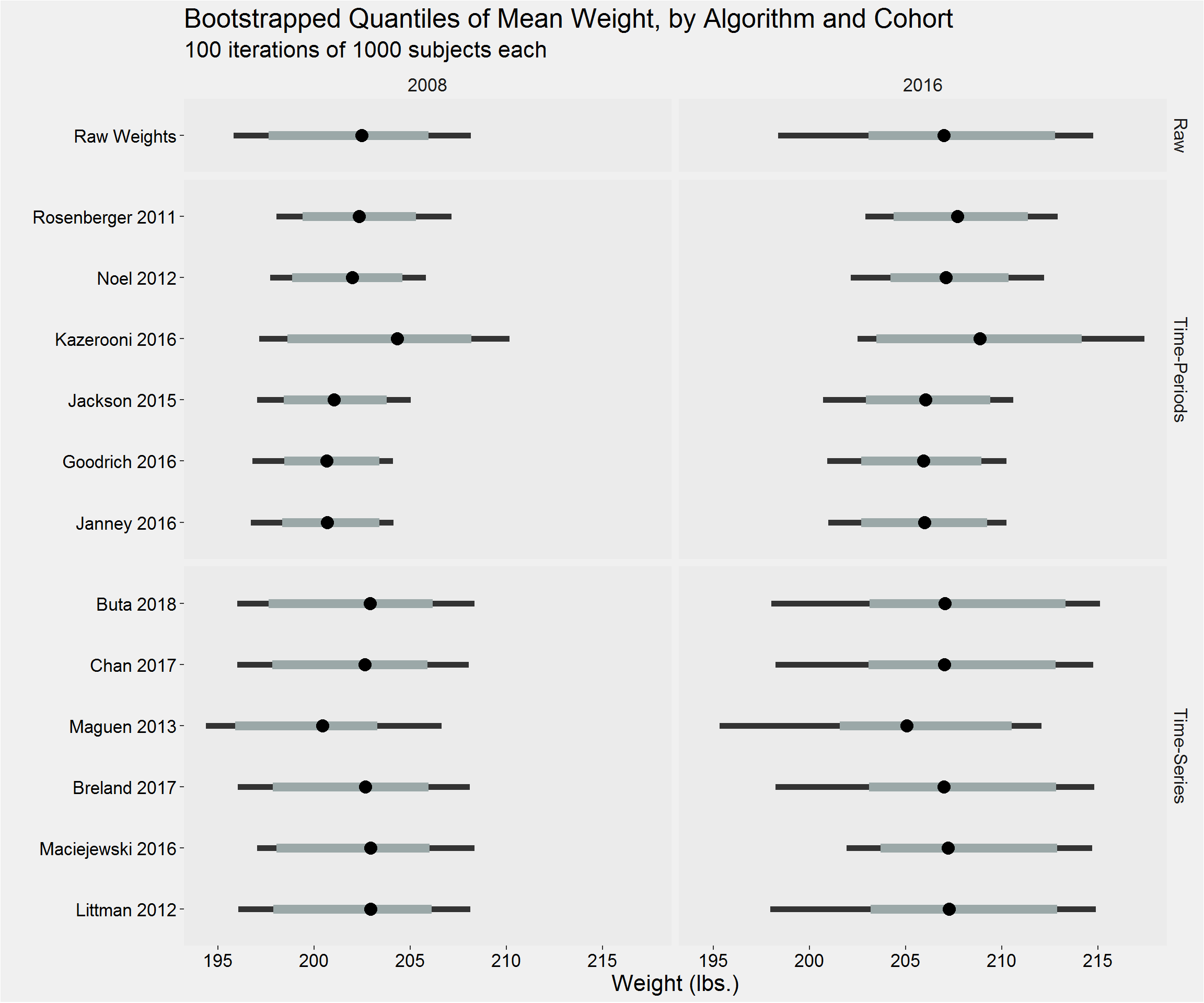
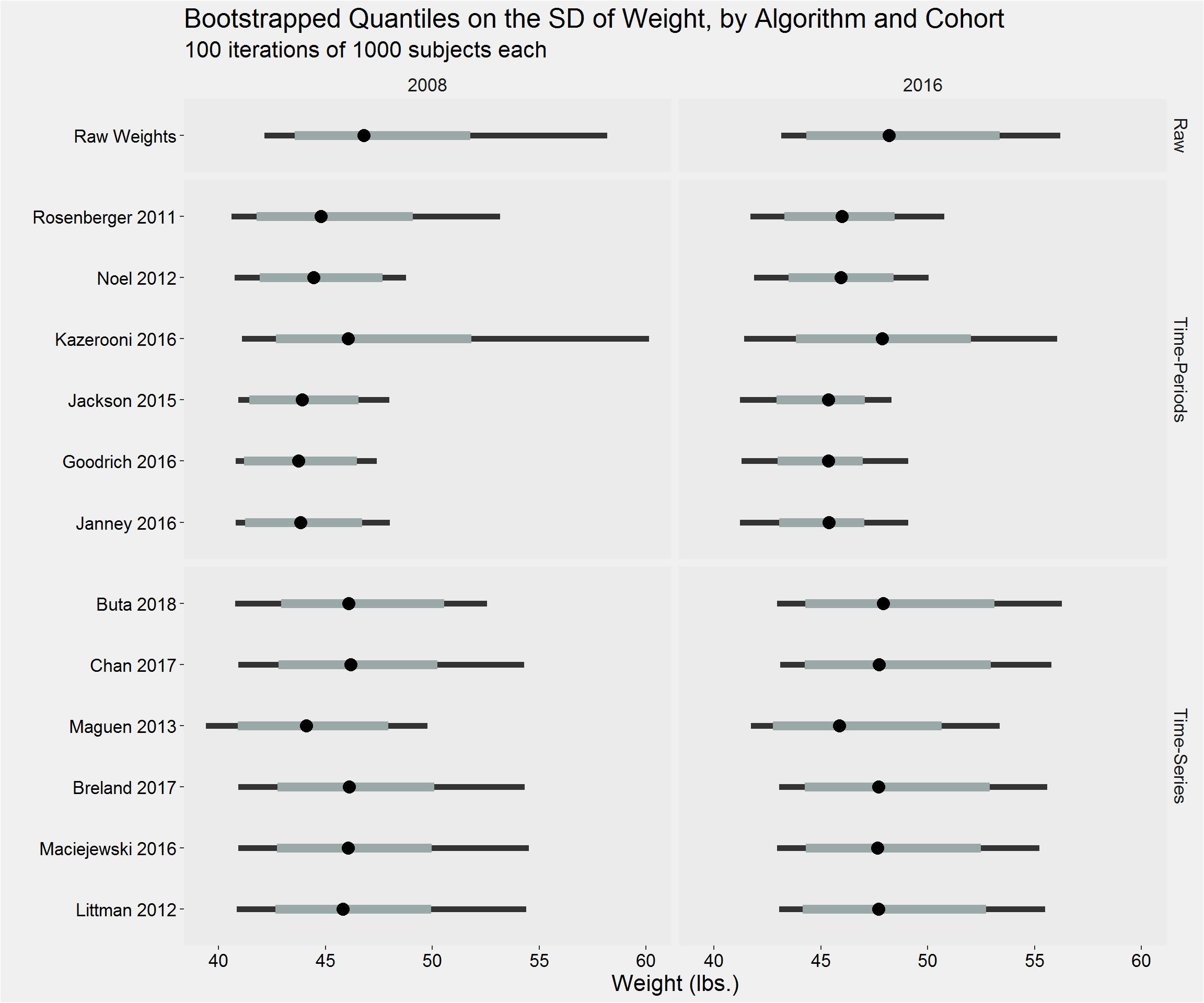
Bootstrapped Estimates

pts <- unique(DF$PatientICN)

N <- 100
weight_samps <- vector("list", N)
key_cols <- c("Algorithm", "Cohort")

pb <- txtProgressBar(min = 0, max = N, initial = 0, style = 3)

for (i in 1:N) {
  setTxtProgressBar(pb, i)
  samp <- sample(pts, 1000, replace = TRUE)
  weight_samps[[i]] <- DF %>% filter(PatientICN %in% samp)
  setDT(weight_samps[[i]])
  setkeyv(weight_samps[[i]], key_cols)
  weight_samps[[i]] <- 
    weight_samps[[i]][, 
                      list(mean = mean(Weight), SD = sd(Weight)), 
                      by = key_cols
                      ]
}

Visualization

Distribution of the mean

Distribution of the sample standard deviation

Alternative, ridgeline plot