Jackson 2015
Excerpt from published methods
BMI was assessed using clinically recorded weight and height, after excluding implausible values (approximately 0.1%)…Weight was recorded as the patient’s baseline weight, and follow-up weights as average weight within subsequent time windows (6 mo: 3–9 mo; 12 mo: 9–15 mo; 24 mo: 21–27 mo; 36 mo: 33–39 mo).
Translation in pseudocode
Unable to tell if they excluded implausible weights before or after defining windows. Also, our samples only collected data 2 years from some baseline point and this algorithm/approach relies on data for up to 3 years. We will build the algorithm only up to 24 months.
DEFINE time t_ijk for person i IN 1:I, j weights IN 1:J {0mo., 6mo., 12 mo., 24mo., 36mo.}, k measurments IN 1:K
FOR i IN 1:I
    weight_i1 := weight @ t_i1 (baseline)
    FOR j IN 2:J
        FOR k IN 1:K
            weight_ijk := all k weights between t_ij +/- 90 days
        END FOR
        IF (weight_ij < 75 lbs OR weight_ij > 700 lbs.)
          weight_ij := NA
        weight_ij := MEAN({weight_ijk})
    END FOR
END FOR
Algorithm in R Code
#' @title Jackson 2015 Measurment Cleaning Algorithm
#' @param DF object of class `data.frame`, containing `id` and `measures`
#' @param id string corresponding to the name of the column of patient identifers in `DF`
#' @param measures string corresponding to the name of the column of measurements in `DF`
#' @param tmeasures string corresponding to the name of the column of measurement collection dates or times in `DF`. If `tmeasures` is a date object, there may be more than one weight on the same day, if it precise datetime object, there may not be more than one weight on the same day
#' @param startPoint string corresponding to the name of the column in `DF` holding the time at which subsequent measurement dates will be assessed, should be the same for each person. Eg., if t = 0 (t[1]) corresponds to an index visit held by the variable 'VisitDate', then startPoint should be set to 'VisitDate'
#' @param outliers numeric vector corresponding to the upper and lower bound for each time entry. Default is `c(75, 700)`.
#' @param t numeric vector of time points to collect measurements, eg. `c(0, 182.5, 365)` for measure collection at t = 0, t = 180 (6 months from t = 0), and t = 365 (1 year from t = 0). Default is `c(0, 182, 365, 730)` according to Jackson et al. 2015
#' @param windows numeric vector of measurement collection windows to use around each time point in `t`. Eg. Jackson et al. 2015 use `c(1, 90, 90, 90)` for t of `c(0, 182.5, 365, 730)`, implying that the closest measurement t = 0 will be collected on the day of the startPoint. Subsequent measurements will be collected 90 days prior to and 90 days post t0+182.5 days, t0+365 days, and t0+730 days.
Jackson2015.f <- function(DF,
                          id,
                          measures,
                          tmeasures,
                          startPoint,
                          t = c(0, 182, 365, 730),
                          windows = c(1, 90, 90, 90),
                          outliers = c(75, 700)) {

  if (!require(dplyr))      install.packages("dplyr")
  if (!require(data.table)) install.packages("data.table")

  tryCatch(
    if (!is.numeric(DF[[measures]])) {
      stop(
        print("measure data must be a numeric vector")
      )
    }
  )

  tryCatch(
    if (!is.numeric(outliers)) {
      stop(
        print("outliers must be numeric")
      )
    }
  )

  tryCatch(
    if (class(DF[[tmeasures]])[1] != class(DF[[startPoint]])[1]) {
      stop(
            print(
                  paste0("date type of tmeasures (",
                  class(DF[[tmeasures]]),
                  ") != date type of startPoint (",
                  class(DF[[startPoint]])[1],
                  ")"
                 )
          )
      )
    }
  )

  tryCatch(
    if (class(t) != "numeric") {
      stop(
        print("t parameter must be a numeric vector")
      )
    }
  )

  tryCatch(
    if (class(windows) != "numeric") {
      stop(
        print("windows parameter must be a numeric vector")
      )
    }
  )

  # convert to data.table
  DT <- data.table::as.data.table(DF)
  data.table::setkeyv(DT, id)

  # Step 1: Set outliers to NA
  DT[,
     output := ifelse(get(measures) < outliers[1]
                      | get(measures) > outliers[2],
                      NA,
                      get(measures))
     ]

  # Step 2: Set windows
  DT[,
     time := as.numeric(difftime(get(tmeasures),
                                 get(startPoint),
                                 tz = "UTC",
                                 units = "days"))
     ]

  # loop through each time point in `t`, place into list
  meas_tn <- vector("list", length(t)) # set empty list
  for (i in 1:length(t)) {

    x <- DT[time >= (t[i] - windows[i]) & time <= (t[i] + windows[i]), ]

    meas_tn[[i]] <- x %>%
      as.data.frame() %>%
      select(eval(id), time, output, !!tmeasures, !!startPoint) %>%
      mutate(measureTime = paste0("t_", t[i]))
  }

  # calculate average weight per measureTime/window
  DT <- data.table::setDT(do.call(rbind, meas_tn))

  key_cols <- c(id, "measureTime")
  data.table::setkeyv(DT, key_cols)
  DT <- DT[,
           list(n = .N, mean = mean(output, na.rm = TRUE)),
           keyby = key_cols
           ][!is.nan(mean) | !is.na(mean)]

  DT <- DT %>% rename(output = mean)
  DT
}
Algorithm in SAS Code
Example in R
Jackson2015.df <- Jackson2015.f(DF,
id = "PatientICN",
measures = "Weight",
tmeasures = "WeightDateTime",
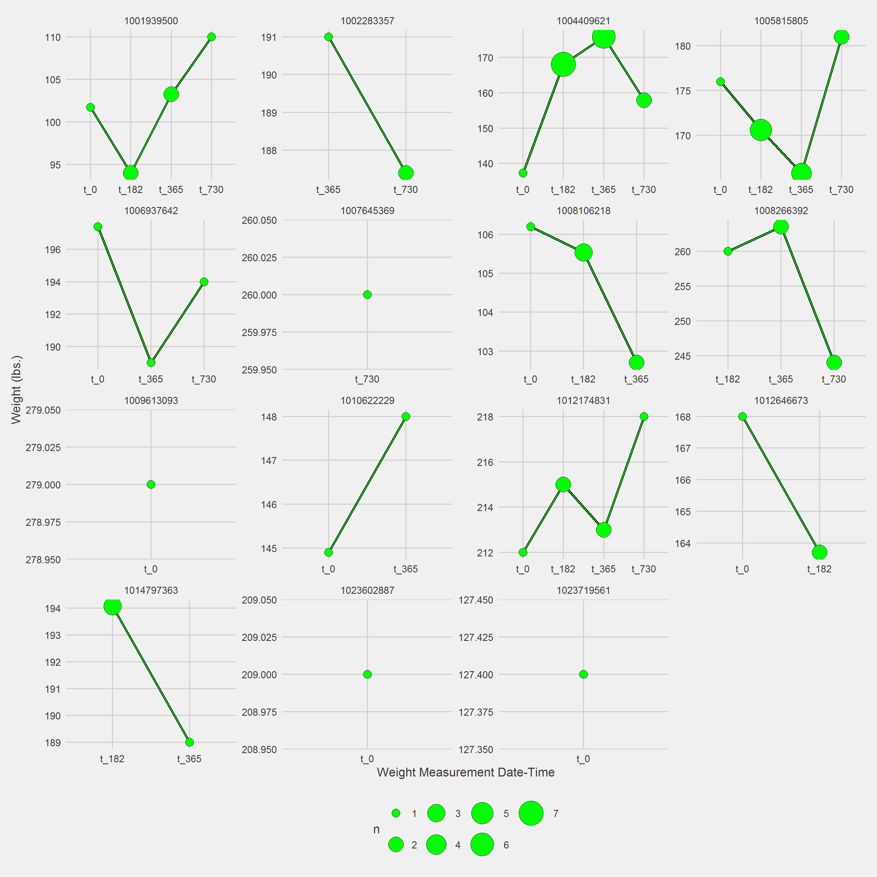
startPoint = "VisitDateTime")Displaying a Vignette of 16 selected patients with at least 1 weight observation removed.
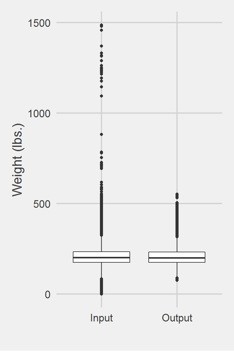
Distribution of Weight Measurements between Raw and Algorithm-Processed Values
 Descriptive statistics by group
group: Input
   vars       n   mean   sd median trimmed   mad min    max  range skew
X1    1 1175995 207.82 48.6  202.3  204.62 44.18   0 1486.2 1486.2 0.98
   kurtosis   se
X1      5.6 0.04
------------------------------------------------------------
group: Output
   vars      n   mean    sd median trimmed   mad   min max  range skew kurtosis
X1    1 251501 206.31 45.52 201.05  203.32 41.59 75.63 553 477.37  0.8     1.47
     se
X1 0.09
Left boxplot is raw data from 2016, PCP visit subjects while the right boxplot describes the output from running Jackson2015.f()