Maguen 2013
Excerpt from published methods
…For our analysis, we used BMI measurements up to 3 years following the index weight measurement (after the last deployment); the average patient-level BMI was calculated for each 6 month interval starting at the index BMI measurement. Only biologically plausible heights and weights were included in the analyses (> 70 lb and < 700 lb; > 46 in. and < 84 in.). To further improve data quality, all available weight measurements (both pre-deployment and post-deployment) were included in a linear mixed model of BMI over time (with a random intercept and slope for each veteran, adjusted for age and gender), in order to identify and exclude within-patient outliers (absolute value of conditional residual \(\ge\) 10). BMI measurements were retained if they were both biologically plausible and not extreme outliers (16 \(\le\) BMI \(\le\) 52).
For our purposes, we will remove BMI from the process and focus on weights, this should not change anything since BMI is a simple transformation of weight data.
Translation in pseudocode
Original
DEFINE time t_ij for person i IN 1:I, j weights IN 1:J
FOR i IN 1:I
    FOR j IN 1:J
        IF (70 lb. <= weight_ij <= 700 lb.)
            weight_ij := weight @ t_ij
-- For BMI --
        IF(46 in. <= height_ij <= 84 in.)
            height_ij := height @ t_ij
    END FOR
    height_i := MEDIAN({height}_ij)
    FOR j In 1:J
        BMI_ij := power(weight_ij (kg) / height_i (m), 2)
    END FOR
    Compute LMM per person: BMI_ij := (beta_0 + veteran_effect) + (beta_1 + veteran_effect) * time_j + beta_2 * age + beta_3 * gender + e_ij
    IF (abs(\hat{BMI_i} | t, age, gender) >= 10)
        BMI_ij := NA
END FOR
Weight Based Algorithm
DEFINE time t_ij for person i IN 1:I, j weights IN 1:J
FOR i IN 1:I
    FOR j IN 1:J
        IF (70 lb. <= weight_ij <= 700 lb.)
            weight_ij := weight @ t_ij
    END FOR
    Compute LMM per person:
      Weight_ij := (beta_0 + veteran_effect) + (beta_1 + veteran_effect) * time_j + beta_2 * age + beta_3 * gender + e_ij
    IF (abs(\hat{Weight_i} | t, age, gender) >= 10)
        Weight_ij := NA
END FOR
Algorithm in R Code
#' @title Maguen 2013 Measurment Cleaning Algorithm
#' @param DF object of class data.frame, containing id and measures
#' @param id string corresponding to the name of the column of patient IDs in DF
#' @param measures string corresponding to the name of the column of measurements in DF
#' @param tmeasures string corresponding to the name of the column of measurement collection dates or times in DF. If tmeasures is a date object, there may be more than one weight on the same day, if it precise datetime object, there may not be more than one weight on the same day
#' @param outliers object of type 'list' with numeric inputs corresponding to the upper and lower bound for each time entry. Default is list(LB = c(70), UB = c(700))
#' @param variables character vector describing the terms in `DF` to include on the RHS of the internal mixed model. E.g., c("Age", "Gender") would generate a model of the form "`measures` ~ Age + Gender + (1|`id`)"
#' @param ResidThreshold single numeric value to be used as a cut off value for the conditional (response) residual for each measurement. Low values are more conservative.
#' @param ... any number of named arguments for the lme4::lmer model
Maguen2013.f <- function(DF,
                         id,
                         measures,
                         tmeasures,
                         outliers = list(LB = 70, UB = 700),
                         variables,
                         ResidThreshold = 10,
                         ...) {

  if (!require(dplyr))  install.packages("dplyr")
  if (!require(lme4))   install.packages("lme4")

  tryCatch(
    if (!is.numeric(DF[[measures]])) {
      stop(
        print("weight data must be a numeric vector")
      )
    }
  )

  tryCatch(
    if (!is.list(outliers)) {
      stop(
        print("outliers must be placed into a list object")
      )
    }
  )

  # step 1: outliers
  DF <- DF %>%
    mutate(
      Output = ifelse(DF[[measures]] >= outliers$LB
                      & DF[[measures]] <= outliers$UB,
                      DF[[measures]],
                      NA_real_)
    )

  # step 2: linear mixed model

  # add time for random slope term
  id <- rlang::sym(id)
  tmeasures <- rlang::sym(tmeasures)

  DF <- DF %>%
    filter(!is.na(Output)) %>%
    group_by(!!id) %>%
    arrange(!!id, !!tmeasures) %>%
    mutate(t = row_number()) %>%
    ungroup()

  f <- paste(
    "Output",
    paste(
      variables,
      collapse = " + "
    ),
    sep = " ~ "
  )
  f <- paste0(f, " + t", " + (1 + t", " | ", id, ")")
  f <- as.formula(f)
  lmm <- eval(
    bquote(
      lme4::lmer(
        .(f),
        data = DF,
        control = lme4::lmerControl(calc.derivs = FALSE)
      )
    )
  )

  DF$resid <- residuals(lmm) # add conditional residuals at ith level

  DF <- DF %>%
    mutate(
      Output = ifelse(abs(resid) >= ResidThreshold, NA_real_, Output)
    )

  DF
}
Algorithm in SAS Code
Example in R
The linear mixed model with random slope and random intercept takes time to run, especially with larger sample sizes.
Maguen2013.df <- Maguen2013.f(DF,
                              id = "PatientICN",
                              measures = "Weight",
                              tmeasures = "WeightDateTime",
                              variables = c("AgeAtVisit", "Gender"))
Displaying a Vignette of 16 selected patients with at least 1 weight observation removed.
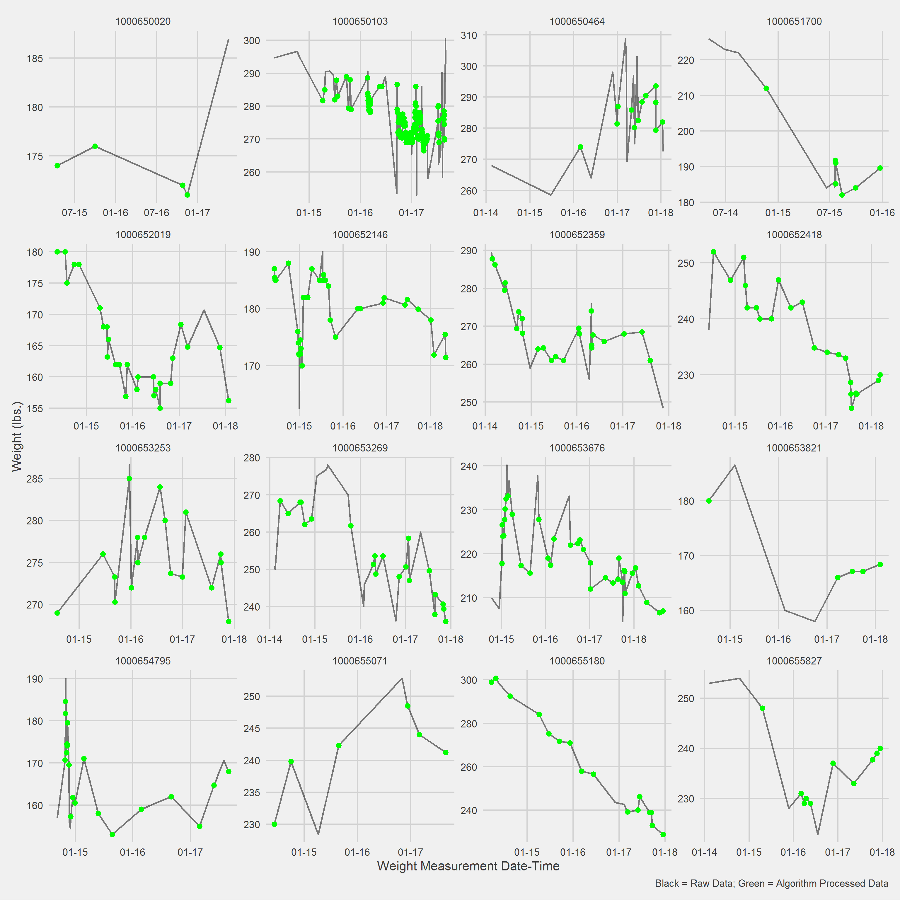
Examining the above, it may make ore sense to include a spline term or some other model that can handle non-linear dynamics; most folks don’t have completely linear weight loss trajectories.
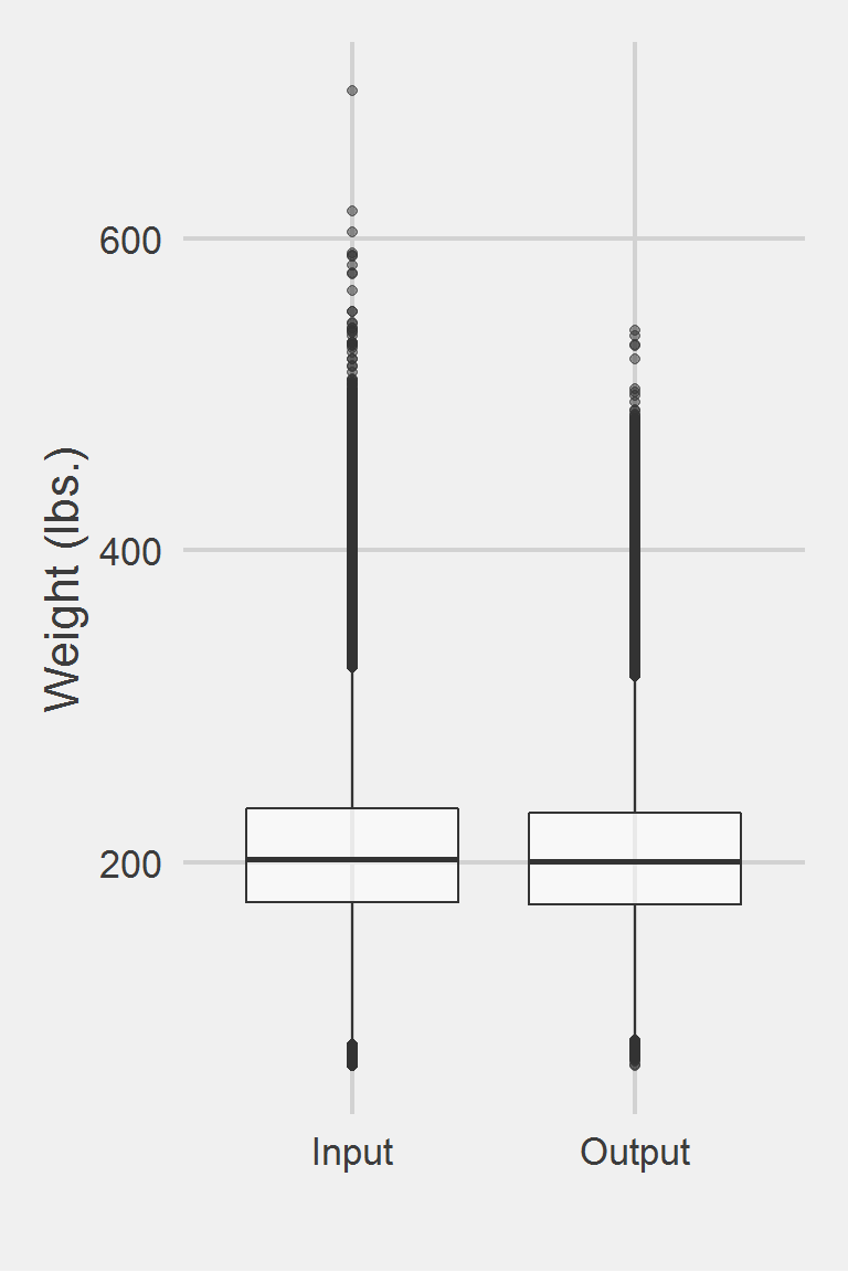
Distribution of raw weight data versus algorithm processed data.
 Descriptive statistics by group
group: Input
   vars       n   mean    sd median trimmed   mad min    max  range skew
X1    1 1175681 207.84 48.31 202.38  204.64 44.15  70 694.46 624.46 0.81
   kurtosis   se
X1     1.46 0.04
------------------------------------------------------------
group: Output
   vars       n   mean    sd median trimmed   mad  min   max range skew
X1    1 1037293 205.58 46.37  200.7  202.69 42.85 70.3 541.1 470.8 0.76
   kurtosis   se
X1     1.29 0.05
Left boxplot is raw data from the same of 2016, PCP visit subjects while the right boxplot describes the output from running Maguen2013.f()