Latent Trajectory Analysis

Sampling 1,000 people from the PCP 2016 Cohort

Trajectory Analysis:

For this analysis we will use a latent class mixed model to examine the effect that different weight cleaning algorithms would have on overall trajectories. Some things to consider: Since this is a linear method it makes the most sense to analyze those individuals where their trajectory is assumed to be decreasing or increasing, and thus this analysis only involves the MOVE 2016 cohort (could also do 2008). Second, based on experience with this data I am only assuming two latent groups or classes, this may not represent reality as people can presumably increase, decrease or maintain the same weight over time. Further analyses is warranted to find a better fitting model.

library(lcmm)

# variable 'subject' must be numeric
for (i in 1:length(me)) {
  if (class(me[[i]]$PatientICN) == "factor") {
    me[[i]]$PatientICN <- as.integer(as.character(me[[i]]$PatientICN))
  }
}

# initial values/model
B <- lcmm(
  Weight ~ time,
  random = ~time,
  subject = "PatientICN",
  ng = 1,
  idiag = TRUE,
  data = me[[1]],
  verbose = TRUE
)

lca.mods <- lapply(
  me,
  FUN = function(x) {
    lcmm(
      Weight ~ time,
      random = ~time,
      subject = "PatientICN",
      mixture = ~time,
      ng = 3,
      idiag = TRUE,
      data = x,
      B = B
    )
  }
)

names(lca.mods) <- names(me)
for (i in 1:length(lca.mods)) lca.mods[[i]]$data <- me[[i]]

Predicted classes

So, there is no guarantee that each class within an algorithms LCMM, will be the same class across algorithms. We can get this information from the signs of the coefficients on “time” in each model.

concept_classes <- c("Loss", "Maintain", "Gain")

traj_edies <- sapply(
  lca.mods,
  function(x) {
    time_coefs <- coef(x)
    which_coef <- grepl("time", names(time_coefs))
    time_coefs <- time_coefs[which_coef]
    traj_class <- sign(round(time_coefs, 3))
    traj_class
  }
) %>%
  reshape2::melt() %>%
  mutate(
    concept_class = case_when(
      value == -1 ~ concept_classes[1],
      value == 0  ~ concept_classes[2],
      value == 1  ~ concept_classes[3]
    ),
    concept_class = factor(
      concept_class,
      levels = concept_classes,
      labels = concept_classes
    ),
    orig_class = case_when(
      Var1 == "time class1" ~ "Class 1",
      Var1 == "time class2" ~ "Class 2",
      Var1 == "time class3" ~ "Class 3"
    ),
    orig_class = factor(orig_class)
  ) %>%
  select(-value, -Var1) %>%
  rename(Algorithm  = Var2)

newdata <- data.frame(time = seq(0, 365, 5))

Ypred_lcmm <- lapply(
  lca.mods,
  function(x) {
    y <- predictY(x, newdata, var.time = "time")
    cbind(y$pred, y$time)
   }
) %>%
  dplyr::bind_rows(.id = "Algorithm") %>%
  reshape2::melt(id.vars = c("Algorithm", "time")) %>%
  mutate(
    Algorithm = factor(Algorithm,
                       levels = names(me),
                       labels = names(me)),
    orig_class = factor(variable,
                        labels = c("Class 1", "Class 2", "Class 3"))
  ) %>%
  select(-variable) %>%
  rename(Ypred = value) %>%
  left_join(
    traj_edies,
    by = c("Algorithm", "orig_class")
  )


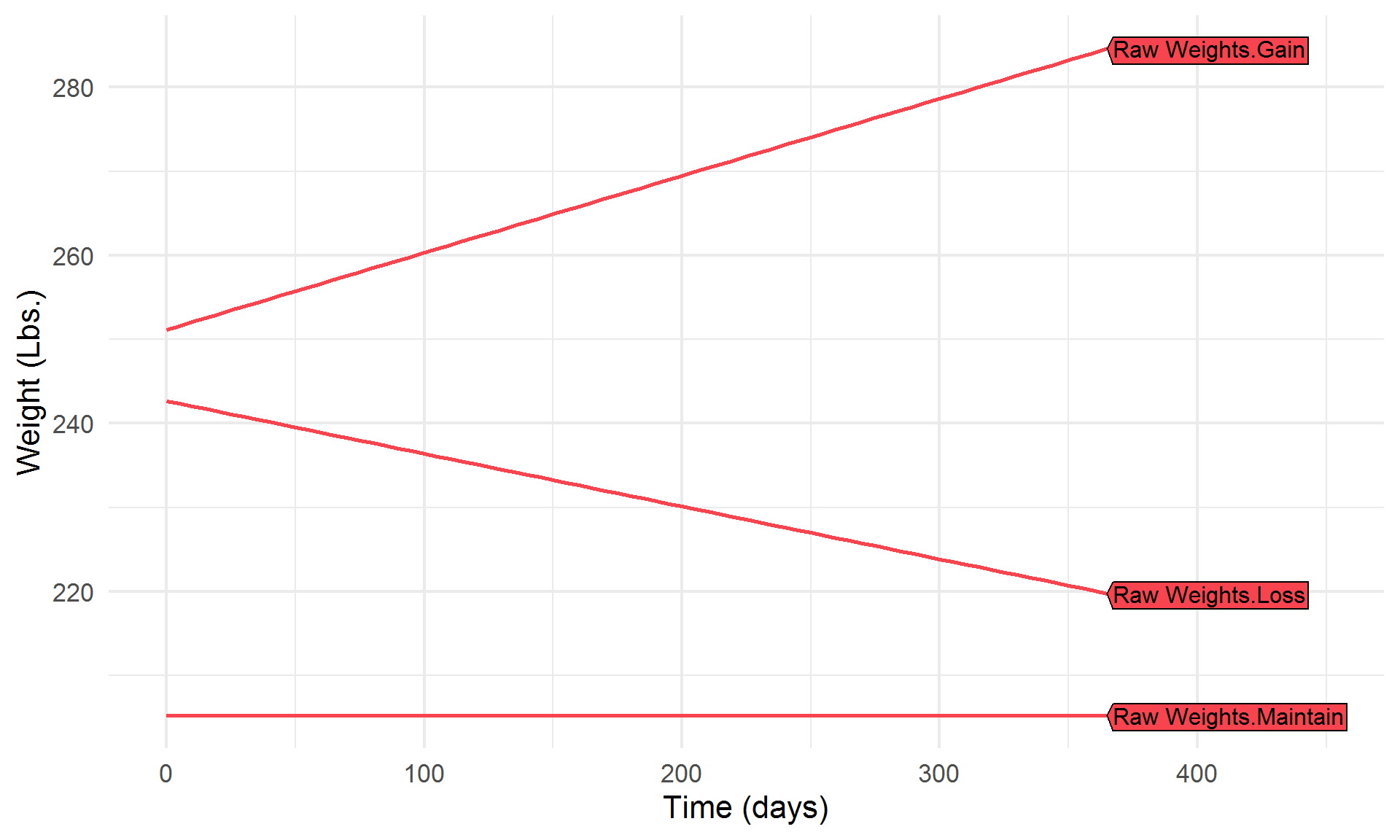
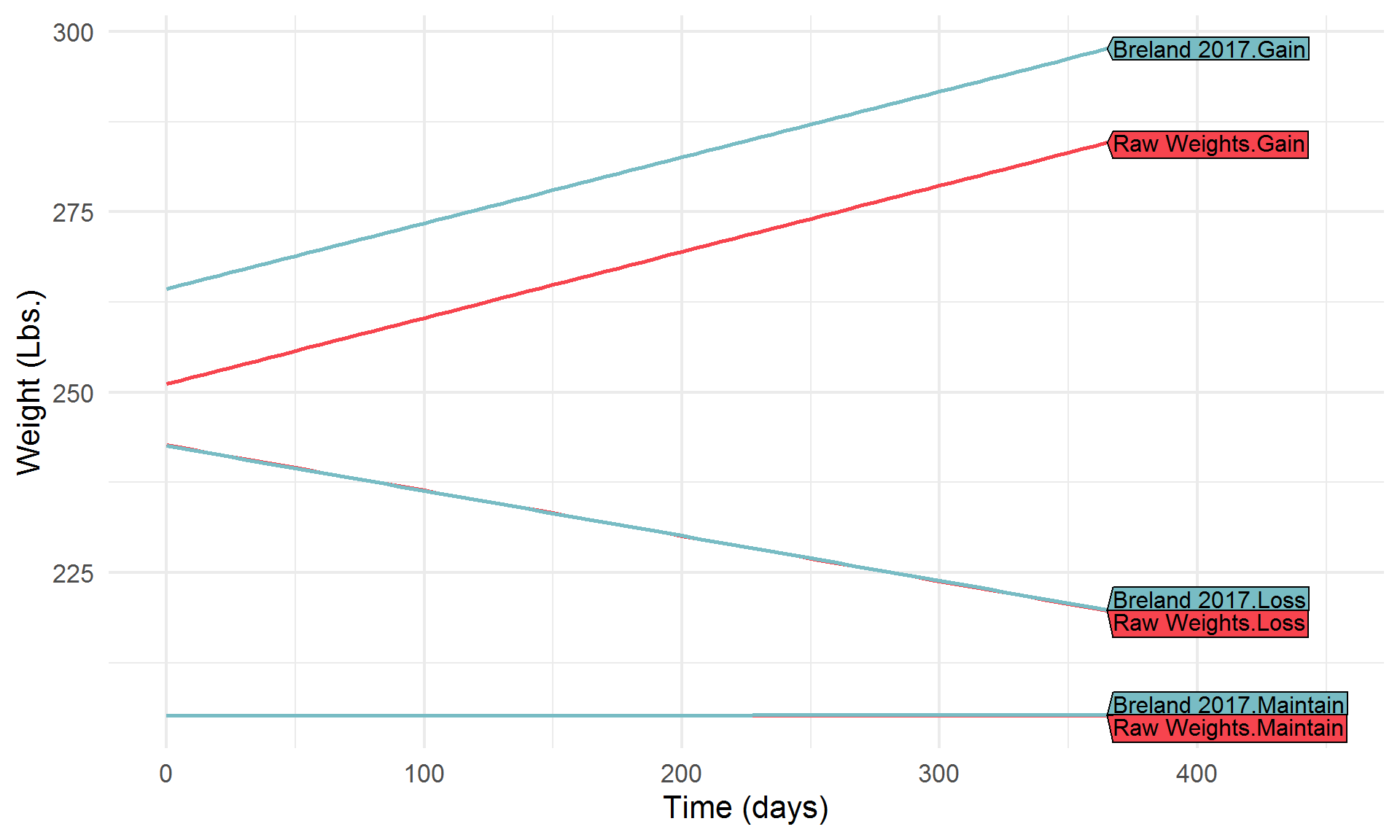
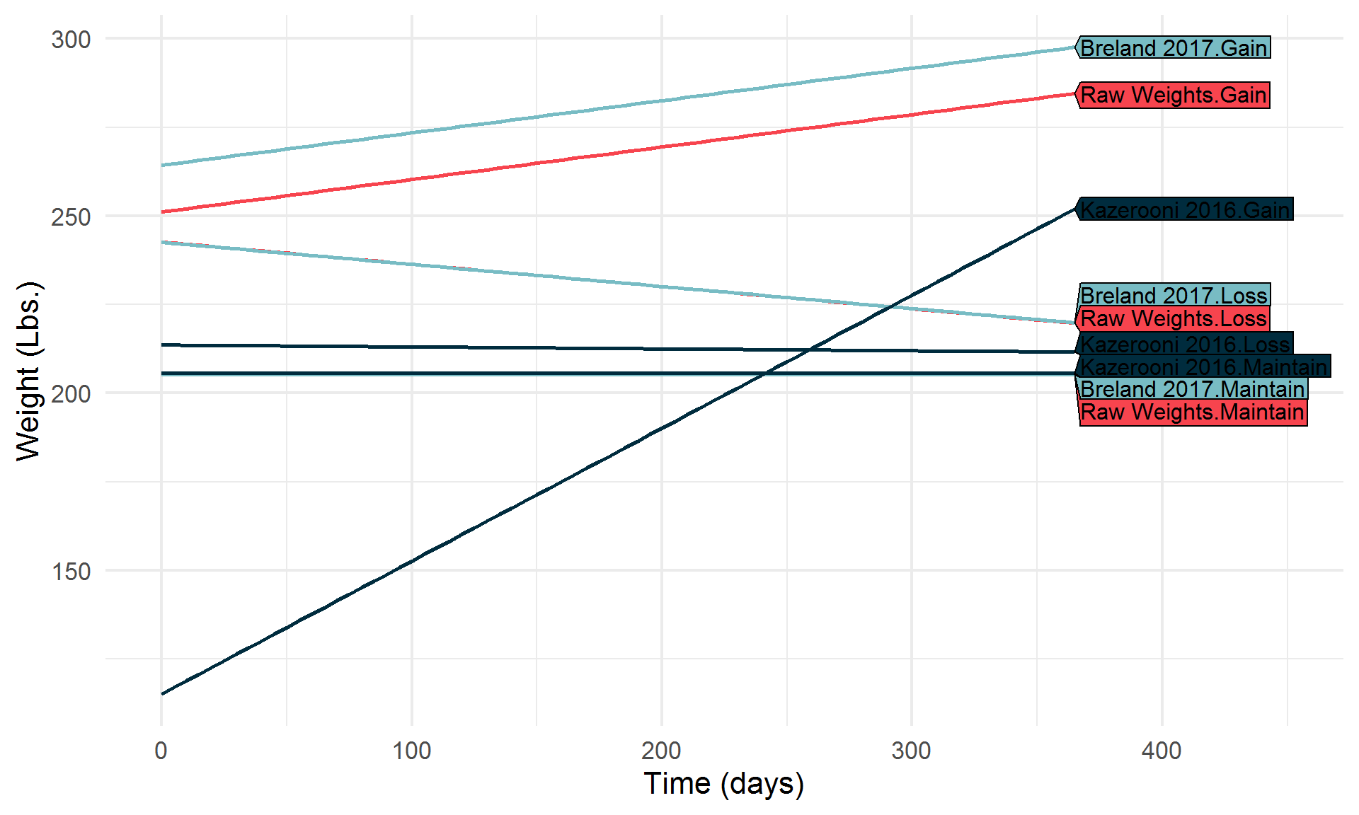
Ypred_lcmm %>%
  ggplot(
    aes(
      x = time, y = Ypred,
      group = interaction(Algorithm, concept_class),
      color = interaction(Algorithm, concept_class)
    )
  ) %>%
  add(geom_line(size = 1)) %>%
  add(theme_fivethirtyeight(16)) %>%
  add(theme(axis.title = element_text(), legend.position = "none")) %>%
  add(xlim(0, 500)) %>% 
  add(directlabels::geom_dl(aes(label = interaction(Algorithm, concept_class)),
                            method = "last.polygons")) %>%
  add(labs(
    x = "Time (days)",
    y = "Weight (Lbs.)",
    title = "Class Specific Mean-Predicted Trajectory",
    subtitle = "2016 Cohort - Latent Class Mixed Model",
    color = ""
  ))

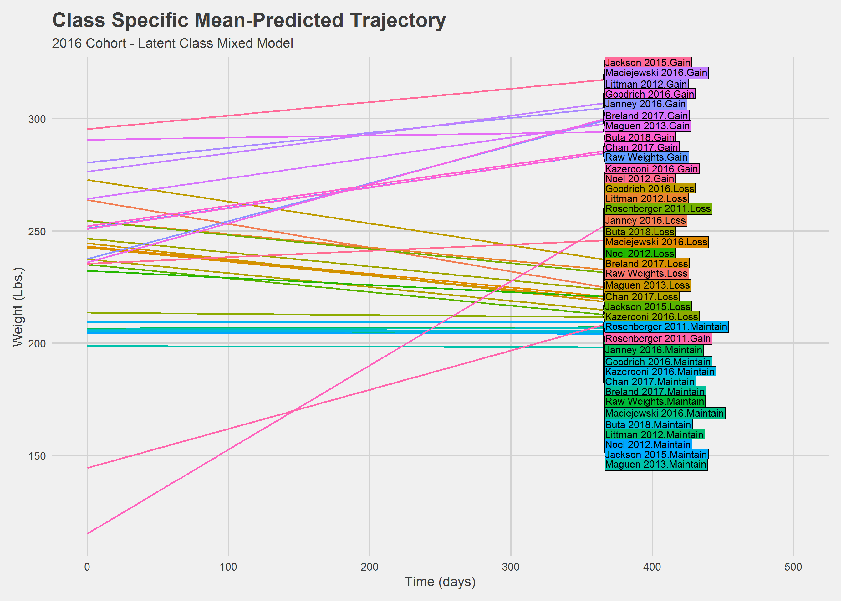
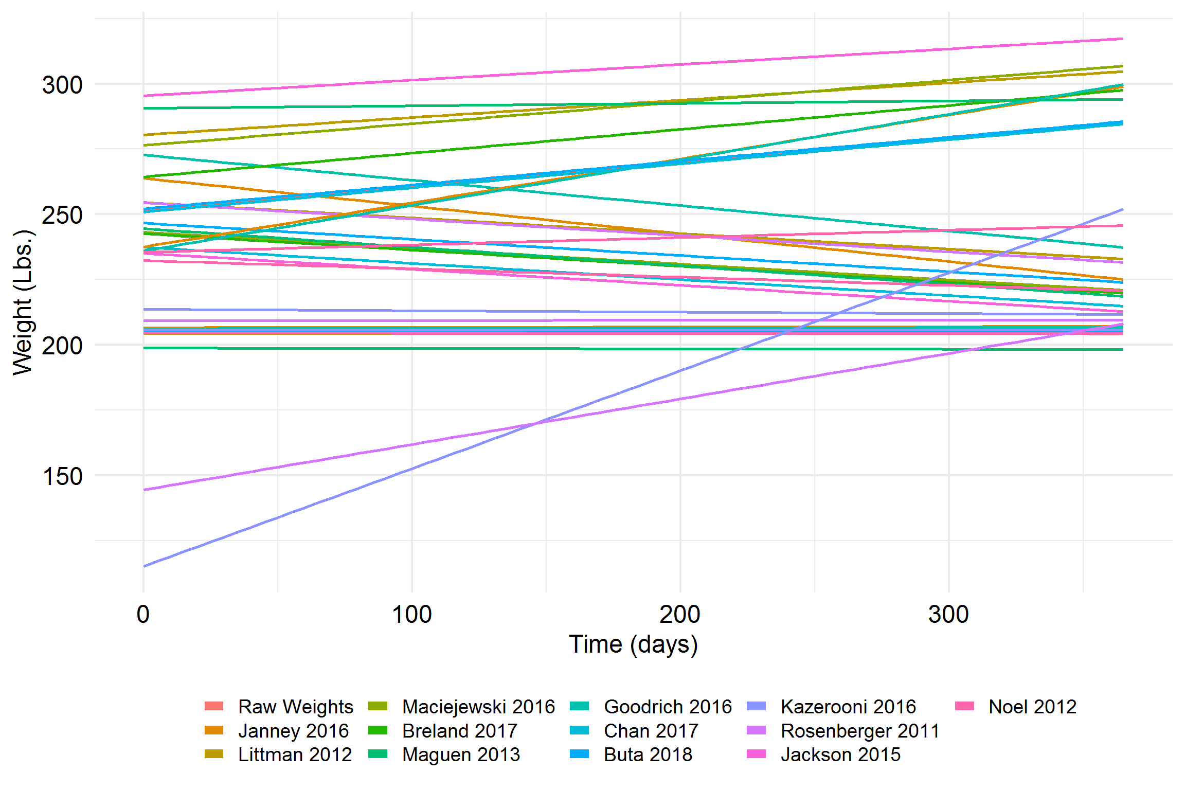
Hah! What a mess. Let’s look at things a little differently.

This next one certainly won’t help anyone,

An Illustration:

library(gganimate)

Ypred_lcmm %>%
  ggplot(
    aes(
      x = time,
      y = Ypred,
      color = Algorithm,
      group = interaction(Algorithm, concept_class)
    )
  ) %>%
  add(geom_line(size = 1)) %>%
  add(theme_minimal(20)) %>%
  add(theme(legend.position = "none")) %>%
  add(labs(
    title = 'Algorithm: {closest_state}',
    x = "Time (days)",
    y = "Weight (lbs.)"
  )) %>%
  add(transition_states(
    states = Algorithm,
    transition_length = 1,
    state_length = 1
  ))

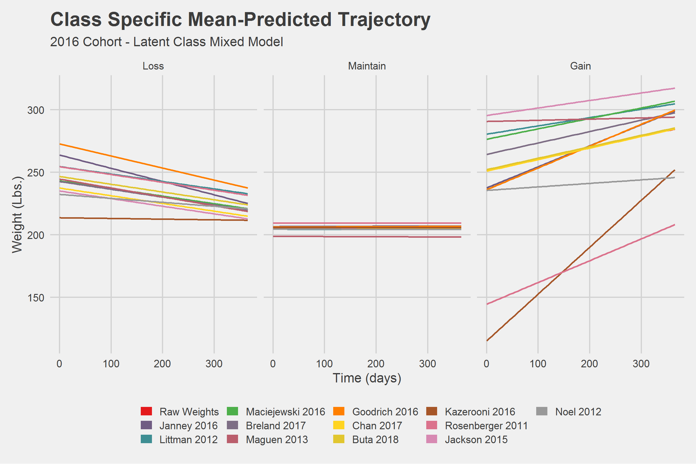
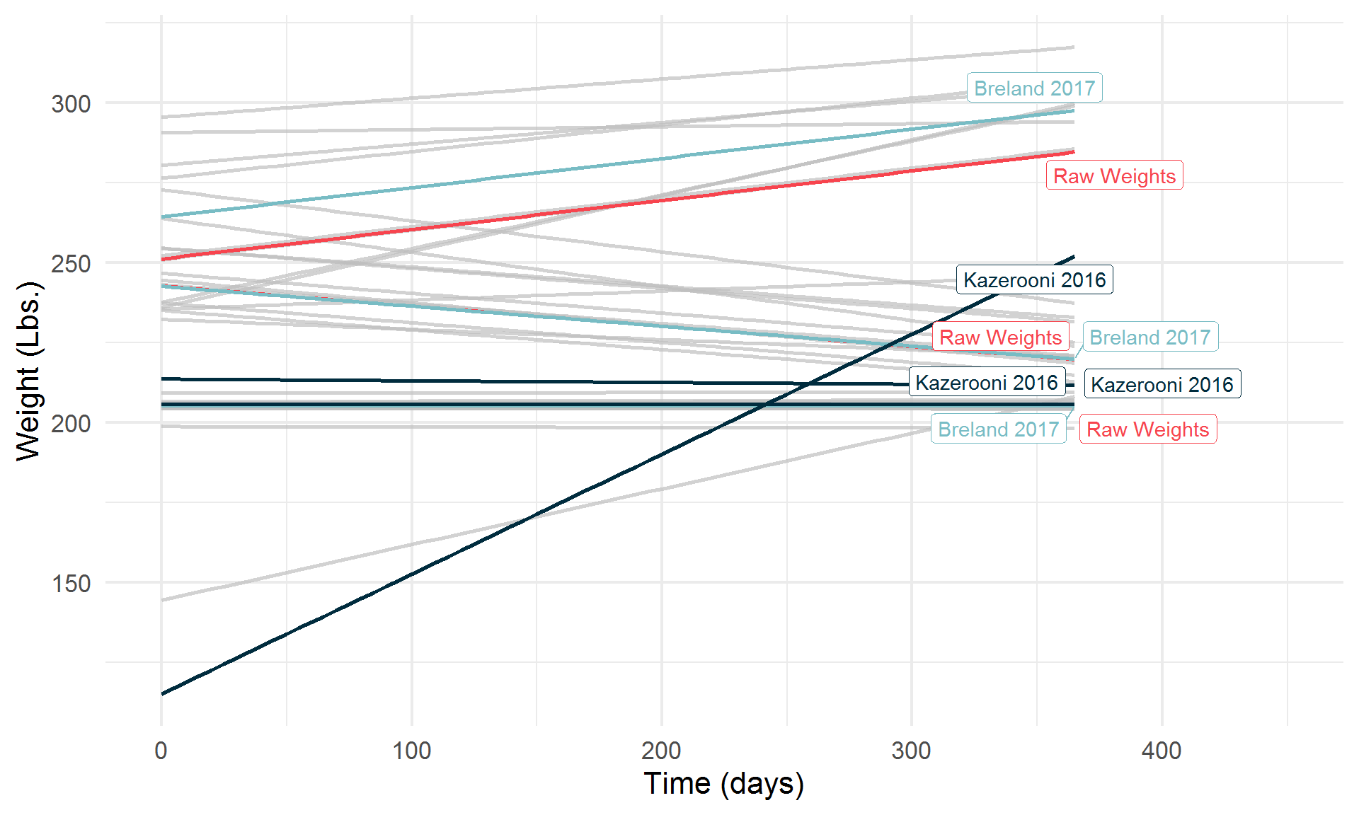
Let’s break it down a bit,

Highlight a few algorithms of interest,

Ypred_lcmm %>%
  ggplot(
      aes(
        x = time,
        y = Ypred,
        group = interaction(Algorithm, concept_class),
        color = Algorithm
      )
  ) %>%
  add(geom_line(size = 1)) %>%
  add(theme_minimal(16)) %>%
  add(theme(axis.title = element_text(), legend.position = "none")) %>%
  add(xlim(0, 450)) %>%
  add(gghighlight::gghighlight(
    Algorithm %in% algos,
    label_key = Algorithm
  )) %>%
  add(scale_color_manual(values = COLS[c(1, 3, 4)])) %>%
  add(labs(
      x = "Time (days)",
      y = "Weight (Lbs.)"
  ))

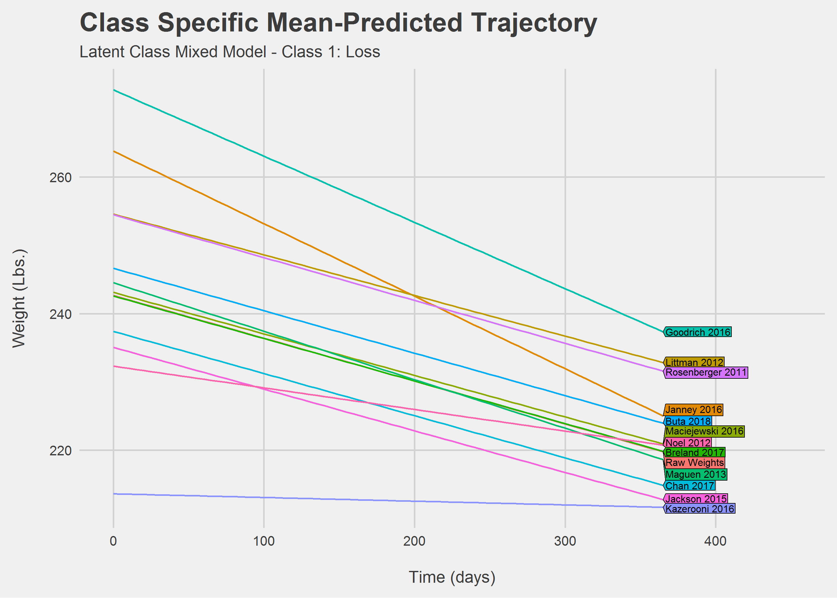
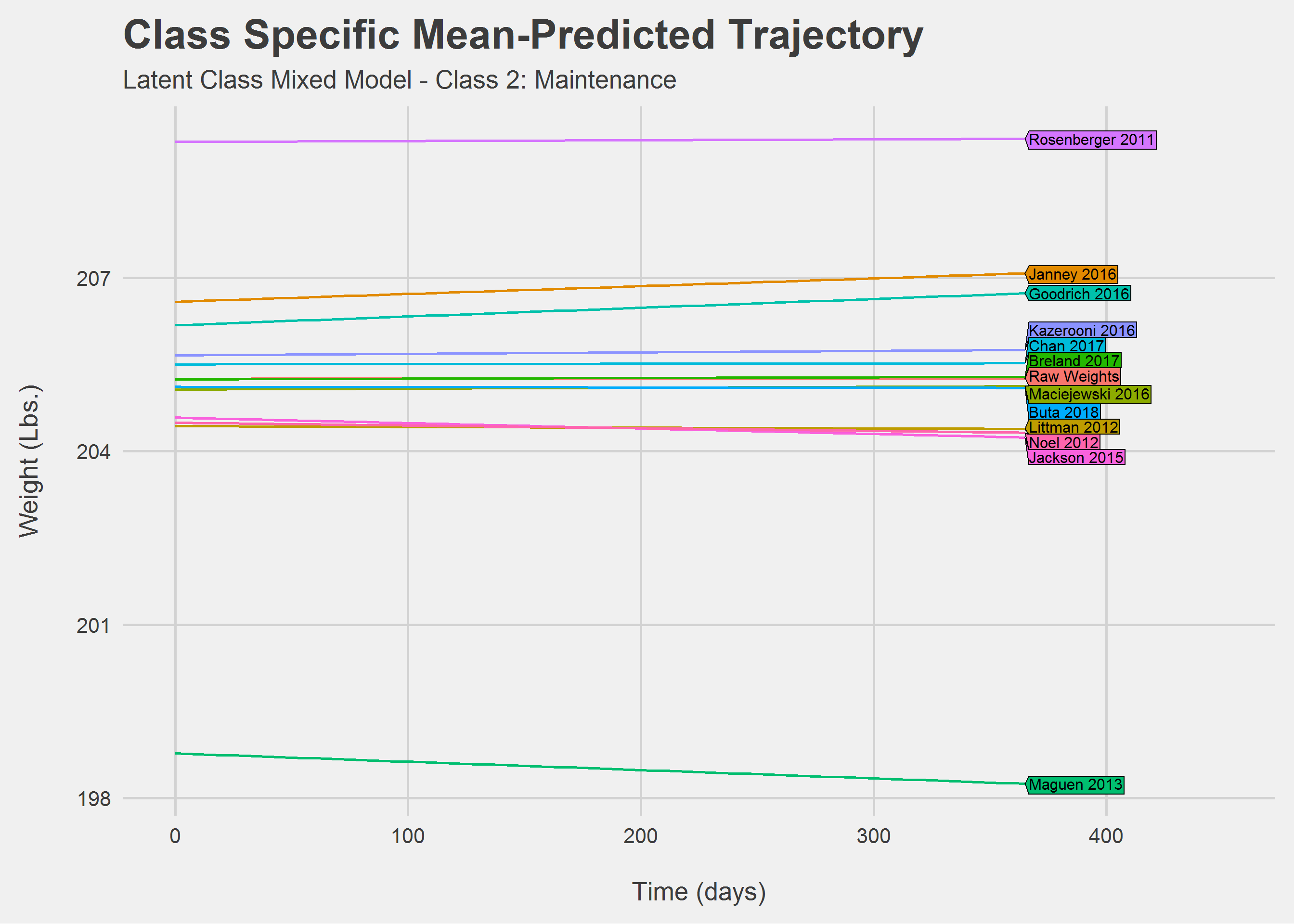
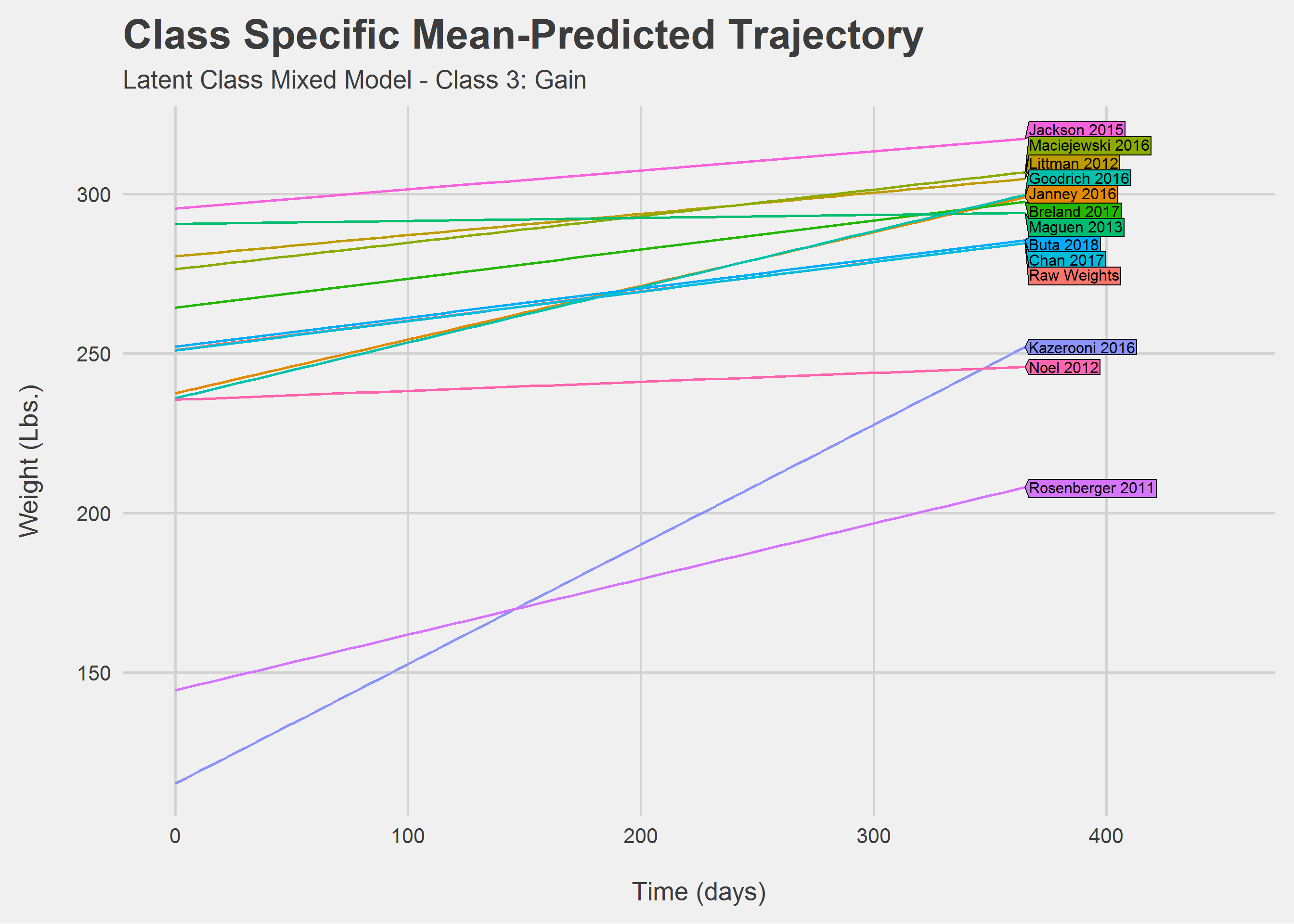
By Class

Looking only at Class 1: Loss

Looking only at Class 2: Maintainence

Looking only at Class 3: Gain

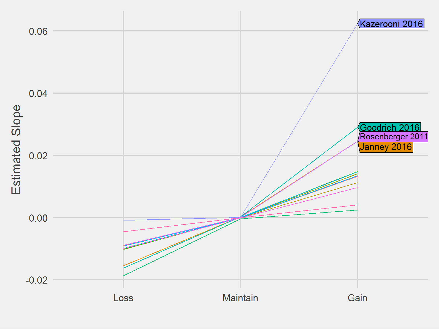
Comparing slopes, numerically

slopes <- sapply(
  lca.mods,
  function(x) {
    time_coefs <- coef(x)
    which_coef <- grepl("time", names(time_coefs))
    time_coefs <- time_coefs[which_coef]
    time_coefs <- round(time_coefs, 5)
    time_coefs
  }
) %>%
  reshape2::melt() %>%
  mutate(
    orig_class = case_when(
      Var1 == "time class1" ~ "Class 1",
      Var1 == "time class2" ~ "Class 2",
      Var1 == "time class3" ~ "Class 3"
    ),
    orig_class = factor(orig_class)
  ) %>%
  select(-Var1) %>%
  rename(Algorithm  = Var2, Slope = value) %>% 
  full_join(traj_edies, by = c("Algorithm", "orig_class"))

slopes %>%
  select(-orig_class) %>%
  select(Algorithm, concept_class, Slope) %>%
  tableStyle(digits = 5)

Algorithm	concept_class	Slope
Raw Weights	Gain	0.01322
Raw Weights	Loss	-0.00906
Raw Weights	Maintain	0.00000
Janney 2016	Maintain	0.00020
Janney 2016	Gain	0.02454
Janney 2016	Loss	-0.01548
Littman 2012	Gain	0.01123
Littman 2012	Loss	-0.01005
Littman 2012	Maintain	-0.00002
Maciejewski 2016	Gain	0.01405
Maciejewski 2016	Loss	-0.01026
Maciejewski 2016	Maintain	0.00003
Breland 2017	Loss	-0.01013
Breland 2017	Gain	0.01482
Breland 2017	Maintain	0.00002
Maguen 2013	Gain	0.00248
Maguen 2013	Maintain	-0.00038
Maguen 2013	Loss	-0.01869
Goodrich 2016	Gain	0.02909
Goodrich 2016	Maintain	0.00025
Goodrich 2016	Loss	-0.01617
Chan 2017	Gain	0.01470
Chan 2017	Loss	-0.00983
Chan 2017	Maintain	0.00001
Buta 2018	Gain	0.01346
Buta 2018	Loss	-0.00913
Buta 2018	Maintain	-0.00001
Kazerooni 2016	Maintain	0.00004
Kazerooni 2016	Loss	-0.00090
Kazerooni 2016	Gain	0.06236
Rosenberger 2011	Gain	0.02456
Rosenberger 2011	Maintain	0.00002
Rosenberger 2011	Loss	-0.00884
Jackson 2015	Maintain	-0.00015
Jackson 2015	Gain	0.00972
Jackson 2015	Loss	-0.00991
Noel 2012	Maintain	-0.00007
Noel 2012	Gain	0.00406
Noel 2012	Loss	-0.00457

algos <- c("Janney 2016", "Goodrich 2016", "Rosenberger 2011", "Kazerooni 2016")

slopes %>%
  ggplot(aes(
    x = concept_class,
    y = Slope,
    group = Algorithm,
    color = Algorithm
  )) %>%
  add(geom_line()) %>%
  add(directlabels::geom_dl(
    data = slopes %>%
      filter(Algorithm %in% algos),
    aes(label = Algorithm),
    method = list("last.polygons")
  )) %>%
  add(theme_fivethirtyeight(16)) %>%
  add(theme(legend.position = "none", axis.title = element_text())) %>%
  add(labs(
    x = "",
    y = "Estimated Slope"
  ))

Membership Posterior Probabilities

For each algorithm weight was modeled with a random slope and intercept. To illustrate the concept, the output from the Raw Weight (non-algorithm) is displayed:

General latent class mixed model 
     fitted by maximum likelihood method 
 
lcmm(fixed = Weight ~ time, mixture = ~time, random = ~time, 
    subject = "PatientICN", ng = 3, idiag = TRUE, data = x)
 
Statistical Model: 
     Dataset: x 
     Number of subjects: 993 
     Number of observations: 7329 
     Number of latent classes: 3 
     Number of parameters: 11  
     Link function: linear  
 
Iteration process: 
     Convergence criteria satisfied 
     Number of iterations:  51 
     Convergence criteria: parameters= 9.6e-05 
                         : likelihood= 2e-06 
                         : second derivatives= 9.8e-07 
 
Goodness-of-fit statistics: 
     maximum log-likelihood: -27768.14  
     AIC: 55558.27  
     BIC: 55612.18  
 
 
Maximum Likelihood Estimates: 
 
Fixed effects in the class-membership model:
(the class of reference is the last class) 

                      coef       Se    Wald p-value
intercept class1  -4.52848  0.34988 -12.943 0.00000
intercept class2  -2.93765  0.22929 -12.812 0.00000

Fixed effects in the longitudinal model:

                                      coef       Se    Wald p-value
intercept class1 (not estimated)         0                         
intercept class2                  -1.22305  2.76107  -0.443 0.65779
intercept class3                  -6.62143  2.47619  -2.674 0.00749
time class1                        0.01322  0.00100  13.272 0.00000
time class2                       -0.00906  0.00067 -13.428 0.00000
time class3                        0.00000  0.00011   0.022 0.98252


Variance-covariance matrix of the random-effects:
          intercept time
intercept  42.42468     
time        0.00000    0

Residual standard error (not estimated) = 1

Parameters of the link function:

                          coef       Se    Wald p-value
Linear 1 (intercept) 251.15091 17.02209  14.754 0.00000
Linear 2 (std err)     6.93123  0.06530 106.151 0.00000

Each class has a slightly different slope on time. The posterior classifications can be examined from each algorithm:

pprobs <- lapply(lca.mods, postprob)

 
Posterior classification: 
  class1 class2 class3
N   9.00  33.00 951.00
%   0.91   3.32  95.77
 
Posterior classification table: 
     --> mean of posterior probabilities in each class 
        prob1  prob2  prob3
class1 0.9631 0.0000 0.0369
class2 0.0000 0.9081 0.0919
class3 0.0015 0.0205 0.9780
 
Posterior probabilities above a threshold (%): 
         class1 class2 class3
prob>0.7 100.00  90.91  98.21
prob>0.8  88.89  84.85  96.64
prob>0.9  88.89  75.76  94.43
 
 
Posterior classification: 
  class1 class2 class3
N 958.00   3.00  14.00
%  98.26   0.31   1.44
 
Posterior classification table: 
     --> mean of posterior probabilities in each class 
        prob1  prob2  prob3
class1 0.9891 0.0013 0.0096
class2 0.0015 0.9985 0.0000
class3 0.1426 0.0000 0.8574
 
Posterior probabilities above a threshold (%): 
         class1 class2 class3
prob>0.7  99.69    100  78.57
prob>0.8  98.96    100  71.43
prob>0.9  97.29    100  57.14
 
 
Posterior classification: 
  class1 class2 class3
N   7.00   32.0 930.00
%   0.72    3.3  95.98
 
Posterior classification table: 
     --> mean of posterior probabilities in each class 
        prob1  prob2  prob3
class1 0.9923 0.0000 0.0077
class2 0.0000 0.8442 0.1558
class3 0.0045 0.0177 0.9778
 
Posterior probabilities above a threshold (%): 
         class1 class2 class3
prob>0.7    100  75.00  98.17
prob>0.8    100  65.62  96.34
prob>0.9    100  59.38  93.66
 
 
Posterior classification: 
  class1 class2 class3
N    7.0  38.00 948.00
%    0.7   3.83  95.47
 
Posterior classification table: 
     --> mean of posterior probabilities in each class 
        prob1  prob2  prob3
class1 0.9847 0.0000 0.0153
class2 0.0000 0.8570 0.1430
class3 0.0017 0.0187 0.9795
 
Posterior probabilities above a threshold (%): 
         class1 class2 class3
prob>0.7    100  76.32  98.31
prob>0.8    100  68.42  97.05
prob>0.9    100  60.53  94.51
 
 
Posterior classification: 
  class1 class2 class3
N  35.00   8.00 950.00
%   3.52   0.81  95.67
 
Posterior classification table: 
     --> mean of posterior probabilities in each class 
        prob1  prob2  prob3
class1 0.8810 0.0000 0.1190
class2 0.0000 0.9684 0.0316
class3 0.0191 0.0014 0.9795
 
Posterior probabilities above a threshold (%): 
         class1 class2 class3
prob>0.7  82.86  100.0  98.21
prob>0.8  77.14  100.0  96.95
prob>0.9  65.71   87.5  94.42
 
 
Posterior classification: 
  class1 class2 class3
N  63.00 902.00  14.00
%   6.44  92.13   1.43
 
Posterior classification table: 
     --> mean of posterior probabilities in each class 
        prob1  prob2  prob3
class1 0.7793 0.2164 0.0043
class2 0.0364 0.9591 0.0045
class3 0.0165 0.1173 0.8662
 
Posterior probabilities above a threshold (%): 
         class1 class2 class3
prob>0.7  66.67  96.34  78.57
prob>0.8  46.03  93.35  57.14
prob>0.9  34.92  87.80  57.14
 
 
Posterior classification: 
  class1 class2 class3
N   3.00 958.00  14.00
%   0.31  98.26   1.44
 
Posterior classification table: 
     --> mean of posterior probabilities in each class 
        prob1  prob2  prob3
class1 0.9983 0.0017 0.0000
class2 0.0012 0.9874 0.0114
class3 0.0000 0.1175 0.8825
 
Posterior probabilities above a threshold (%): 
         class1 class2 class3
prob>0.7    100  99.37  85.71
prob>0.8    100  98.23  71.43
prob>0.9    100  96.97  71.43
 
 
Posterior classification: 
  class1 class2 class3
N   9.00  38.00 922.00
%   0.93   3.92  95.15
 
Posterior classification table: 
     --> mean of posterior probabilities in each class 
        prob1  prob2  prob3
class1 0.9635 0.0000 0.0365
class2 0.0000 0.8557 0.1443
class3 0.0013 0.0175 0.9812
 
Posterior probabilities above a threshold (%): 
         class1 class2 class3
prob>0.7 100.00  76.32  98.48
prob>0.8  88.89  68.42  97.29
prob>0.9  88.89  57.89  95.34
 
 
Posterior classification: 
  class1 class2 class3
N   9.00  33.00 868.00
%   0.99   3.63  95.38
 
Posterior classification table: 
     --> mean of posterior probabilities in each class 
        prob1  prob2  prob3
class1 0.9668 0.0000 0.0332
class2 0.0000 0.8972 0.1028
class3 0.0014 0.0204 0.9782
 
Posterior probabilities above a threshold (%): 
         class1 class2 class3
prob>0.7 100.00  84.85  98.16
prob>0.8  88.89  81.82  96.31
prob>0.9  88.89  72.73  94.47
 
 
Posterior classification: 
  class1 class2 class3
N      0 262.00   1.00
%      0  99.62   0.38
 
Posterior classification table: 
     --> mean of posterior probabilities in each class 
        prob1  prob2 prob3
class1    NaN    NaN   NaN
class2 0.0037 0.9963     0
class3 0.0000 0.0000     1
 
Posterior probabilities above a threshold (%): 
         class1 class2 class3
prob>0.7    NaN    100    100
prob>0.8    NaN    100    100
prob>0.9    NaN    100    100
 
 
Posterior classification: 
  class1 class2 class3
N    2.0  634.0   21.0
%    0.3   96.5    3.2
 
Posterior classification table: 
     --> mean of posterior probabilities in each class 
       prob1  prob2  prob3
class1     1 0.0000 0.0000
class2     0 0.9870 0.0130
class3     0 0.2019 0.7981
 
Posterior probabilities above a threshold (%): 
         class1 class2 class3
prob>0.7    100  98.42  66.67
prob>0.8    100  97.79  57.14
prob>0.9    100  96.21  42.86
 
 
Posterior classification: 
  class1 class2 class3
N 940.00  11.00  26.00
%  96.21   1.13   2.66
 
Posterior classification table: 
     --> mean of posterior probabilities in each class 
        prob1  prob2  prob3
class1 0.9726 0.0081 0.0193
class2 0.0487 0.9510 0.0002
class3 0.1397 0.0000 0.8603
 
Posterior probabilities above a threshold (%): 
         class1 class2 class3
prob>0.7  98.30  90.91  88.46
prob>0.8  96.38  90.91  69.23
prob>0.9  93.51  90.91  53.85
 
 
Posterior classification: 
  class1 class2 class3
N  919.0   35.0   46.0
%   91.9    3.5    4.6
 
Posterior classification table: 
     --> mean of posterior probabilities in each class 
        prob1  prob2  prob3
class1 0.9537 0.0247 0.0216
class2 0.1849 0.8150 0.0002
class3 0.1795 0.0000 0.8205
 
Posterior probabilities above a threshold (%): 
         class1 class2 class3
prob>0.7  96.41  65.71  71.74
prob>0.8  92.82  51.43  65.22
prob>0.9  86.18  40.00  43.48
 

Posterior Classifications, by Algorithm

post_class <- vector("list", length(pprobs))
for(i in seq_along(pprobs)) {
    post_class[[i]] <- reshape2::melt(pprobs[[i]][[1]])
    post_class[[i]]$Algorithm <- names(pprobs)[[i]]
}

post_class %>%
  bind_rows() %>%
  mutate(
    orig_class = case_when(
      Var2 == "class1" ~ "Class 1",
      Var2 == "class2" ~ "Class 2",
      Var2 == "class3" ~ "Class 3"
    )
  ) %>%
  left_join(traj_edies, by = c("Algorithm", "orig_class")) %>%
  select(Algorithm, concept_class, value, Var1) %>%
  reshape2::dcast(Algorithm + concept_class ~ Var1, value.var = "value") %>%
  scrollTable()

Algorithm	concept_class	N	%
Breland 2017	Loss	35	3.52
Breland 2017	Maintain	950	95.67
Breland 2017	Gain	8	0.81
Buta 2018	Loss	33	3.63
Buta 2018	Maintain	868	95.38
Buta 2018	Gain	9	0.99
Chan 2017	Loss	38	3.92
Chan 2017	Maintain	922	95.15
Chan 2017	Gain	9	0.93
Goodrich 2016	Loss	14	1.44
Goodrich 2016	Maintain	958	98.26
Goodrich 2016	Gain	3	0.31
Jackson 2015	Loss	26	2.66
Jackson 2015	Maintain	940	96.21
Jackson 2015	Gain	11	1.13
Janney 2016	Loss	14	1.44
Janney 2016	Maintain	958	98.26
Janney 2016	Gain	3	0.31
Kazerooni 2016	Loss	262	99.62
Kazerooni 2016	Maintain	0	0.00
Kazerooni 2016	Gain	1	0.38
Littman 2012	Loss	32	3.30
Littman 2012	Maintain	930	95.98
Littman 2012	Gain	7	0.72
Maciejewski 2016	Loss	38	3.83
Maciejewski 2016	Maintain	948	95.47
Maciejewski 2016	Gain	7	0.70
Maguen 2013	Loss	14	1.43
Maguen 2013	Maintain	902	92.13
Maguen 2013	Gain	63	6.44
Noel 2012	Loss	46	4.60
Noel 2012	Maintain	919	91.90
Noel 2012	Gain	35	3.50
Raw Weights	Loss	33	3.32
Raw Weights	Maintain	951	95.77
Raw Weights	Gain	9	0.91
Rosenberger 2011	Loss	21	3.20
Rosenberger 2011	Maintain	634	96.50
Rosenberger 2011	Gain	2	0.30

meanPP <- vector("list", length(pprobs))
for(i in seq_along(pprobs)) {
    meanPP[[i]] <- reshape2::melt(pprobs[[i]][[2]])
    meanPP[[i]]$Algorithm <- names(pprobs)[[i]]
}

meanPP %>%
  bind_rows() %>%
  mutate(
    orig_class = case_when(
      Var1 == "class1" ~ "Class 1",
      Var1 == "class2" ~ "Class 2",
      Var1 == "class3" ~ "Class 3"
    )
  ) %>%
  left_join(traj_edies, by = c("Algorithm", "orig_class")) %>%
  select(Algorithm, concept_class, value, Var2) %>%
  rename(cProb = Var2) %>%
  reshape2::dcast(Algorithm + cProb ~ concept_class, value.var = "value") %>%
  scrollTable()

Algorithm	cProb	Loss	Maintain	Gain
Breland 2017	prob1	0.88	0.02	0.00
Breland 2017	prob2	0.00	0.00	0.97
Breland 2017	prob3	0.12	0.98	0.03
Buta 2018	prob1	0.00	0.00	0.97
Buta 2018	prob2	0.90	0.02	0.00
Buta 2018	prob3	0.10	0.98	0.03
Chan 2017	prob1	0.00	0.00	0.96
Chan 2017	prob2	0.86	0.02	0.00
Chan 2017	prob3	0.14	0.98	0.04
Goodrich 2016	prob1	0.00	0.00	1.00
Goodrich 2016	prob2	0.12	0.99	0.00
Goodrich 2016	prob3	0.88	0.01	0.00
Jackson 2015	prob1	0.14	0.97	0.05
Jackson 2015	prob2	0.00	0.01	0.95
Jackson 2015	prob3	0.86	0.02	0.00
Janney 2016	prob1	0.14	0.99	0.00
Janney 2016	prob2	0.00	0.00	1.00
Janney 2016	prob3	0.86	0.01	0.00
Kazerooni 2016	prob1	0.00	NaN	0.00
Kazerooni 2016	prob2	1.00	NaN	0.00
Kazerooni 2016	prob3	0.00	NaN	1.00
Littman 2012	prob1	0.00	0.00	0.99
Littman 2012	prob2	0.84	0.02	0.00
Littman 2012	prob3	0.16	0.98	0.01
Maciejewski 2016	prob1	0.00	0.00	0.98
Maciejewski 2016	prob2	0.86	0.02	0.00
Maciejewski 2016	prob3	0.14	0.98	0.02
Maguen 2013	prob1	0.02	0.04	0.78
Maguen 2013	prob2	0.12	0.96	0.22
Maguen 2013	prob3	0.87	0.00	0.00
Noel 2012	prob1	0.18	0.95	0.18
Noel 2012	prob2	0.00	0.02	0.82
Noel 2012	prob3	0.82	0.02	0.00
Raw Weights	prob1	0.00	0.00	0.96
Raw Weights	prob2	0.91	0.02	0.00
Raw Weights	prob3	0.09	0.98	0.04
Rosenberger 2011	prob1	0.00	0.00	1.00
Rosenberger 2011	prob2	0.20	0.99	0.00
Rosenberger 2011	prob3	0.80	0.01	0.00