Weight Change Comparison
Patient-Level
Often, the metric studied in weight loss studies performed within the VA use “Weight loss \(\geq\) 5% of baseline,” where baseline is defined as any weight measurement taken within 60 days of some arbitrary baseline date (or time point) and 1-year follow-up measure taken within 1 year of the baseline date +/- 60 days. We will apply the algorithms to the PCP cohort from 2008 and 2016 and then collect weights for the weight loss measurements. After some deliberation, we have also decided to analyze weight gain, i.e., \(\geq\) 5% weight gain from baseline weight.
# Raw Data
vars <- c("PatientICN", "Sta3n", "Weight", "measureTime")
raw <- lapply(weight.ls, function(x) timePoints.f(x) %>% select(all_of(vars)))
raw <- bind_rows(raw, .id = "Cohort")

#--------------------------------- Janney 2016 -------------------------------#

janney2016.df <- lapply(
  weight.ls,
  FUN = function(x) {
    Janney2016.f(
      DF = x,
      id = "PatientICN",
      measures = "Weight",
      tmeasures = "WeightDateTime",
      startPoint = "VisitDateTime"
    ) %>%
    filter(!is.na(Weight_OR)) %>%
    select(
      PatientICN,
      Sta3n,
      WeightDateTime,
      VisitDateTime,
      Weight_OR
    ) %>%
    rename(Weight = Weight_OR) %>%
    timePoints.f() %>%
    select(all_of(vars))
  }
) %>%
  bind_rows(.id = "Cohort")

#-------------------------------- Littman 2012 -------------------------------#

littman2012.df <- lapply(
  weight.ls,
  FUN = function(x) {
    Littman2012.f(
      DF = x,
      id = "PatientICN",
      measures = "Weight",
      tmeasures = "WeightDateTime"
    ) %>%
      select(
        PatientICN,
        Sta3n,
        VisitDateTime,
        OutputMeasurement,
        WeightDateTime
      ) %>%
      filter(!is.na(OutputMeasurement)) %>%
      rename(Weight = OutputMeasurement) %>%
      timePoints.f() %>%
      select(all_of(vars))
  }
) %>%
  bind_rows(.id = "Cohort")

#------------------------------ Maciejewski 2016 -----------------------------#

maciejewski2016.2008 <- maciejewski %>%
  filter(SampleYear == "2008" & IO == "Output") %>%
  mutate(PatientICN = as.character(PatientICN)) %>%
  left_join(
    weight.ls[["PCP2008"]] %>%
      distinct(PatientICN, Sta3n),
    by = "PatientICN"
  ) %>%
  mutate(
    WeightDateTime = lubridate::as_datetime(WeightDate, tz = "UTC"),
    Sta3n = factor(Sta3n)
  ) %>%
  select(-IO, -WeightDate, -SampleYear)

maciejewski2016.2016 <- maciejewski %>%
  filter(SampleYear == "2016" & IO == "Output") %>%
  mutate(PatientICN = as.character(PatientICN)) %>%
  left_join(
    weight.ls[["PCP2016"]] %>%
      distinct(PatientICN, Sta3n),
    by = "PatientICN"
  ) %>%
  mutate(
    WeightDateTime = lubridate::as_datetime(WeightDate, tz = "UTC"),
    Sta3n = factor(Sta3n)
  ) %>%
  select(-IO, -WeightDate, -SampleYear)

maciejewski2016.ls <- list(
  PCP2008 = maciejewski2016.2008,
  PCP2016 = maciejewski2016.2016
)

rm(maciejewski2016.2008, maciejewski2016.2016)

maciejewski2016.df <- lapply(
  maciejewski2016.ls,
  FUN = function(x) {
    windows.f(
      DF = x,
      id = "PatientICN",
      measures = "Weight",
      tmeasures = "WeightDateTime",
      startPoint = "VisitDateTime",
      t = c(0, 365),
      windows = c(60, 60)
    ) %>%
   select(all_of(vars))
  }
) %>%
  bind_rows(.id = "Cohort")

rm(maciejewski2016.ls)

#-------------------------------- Breland 2017 --------------------------------#

breland2017.df <- lapply(
  weight.ls,
  FUN = function(x) {
    Breland2017.f(
      DF = x,
      id = "PatientICN",
      measures = "Weight",
      tmeasures = "WeightDateTime"
    ) %>%
    filter(!is.na(measures_aug_)) %>%
    select(
      PatientICN,
      Sta3n,
      VisitDateTime,
      WeightDateTime,
      measures_aug_
    ) %>%
    rename(Weight = measures_aug_) %>%
    timePoints.f() %>%
    select(all_of(vars))
  }
) %>%
  bind_rows(.id = "Cohort")

#-------------------------------- Maguen 2013 --------------------------------#

maguen2013.df <- lapply(
  weight.ls,
  FUN = function(x) {
    Maguen2013.f(
      DF = x,
      id = "PatientICN",
      measures = "Weight",
      tmeasures = "WeightDateTime",
      variables = c("AgeAtVisit", "Gender")
    ) %>%
    filter(!is.na(Output)) %>%
    select(
      PatientICN,
      Sta3n,
      VisitDateTime,
      WeightDateTime,
      Output
    ) %>%
    rename(Weight = Output) %>%
    timePoints.f() %>%
    select(all_of(vars))
  }
) %>%
  bind_rows(.id = "Cohort")

#------------------------------- Goodrich 2016 -------------------------------#

goodrich2016.df <- lapply(
  weight.ls,
  FUN = function(x) {
    Goodrich2016.f(
      DF = x,
      id = "PatientICN",
      measures = "Weight",
      tmeasures = "WeightDateTime",
      startPoint = "VisitDateTime"
    ) %>%
    filter(!is.na(output)) %>%
    select(
      PatientICN,
      Sta3n,
      VisitDateTime,
      WeightDateTime,
      output
    ) %>%
    rename(Weight = output) %>%
    timePoints.f() %>%
    select(all_of(vars))
  }
) %>%
  bind_rows(.id = "Cohort")

#----------------------------- Chan & Raffa 2017 -----------------------------#

chan2017.df <- lapply(
  weight.ls,
  FUN = function(x) {
    Chan2017.f(
      DF = x,
      id = "PatientICN",
      measures = "Weight",
      tmeasures = "WeightDateTime"
    ) %>%
    filter(!is.na(measures_aug_)) %>%
    select(
      PatientICN,
      Sta3n,
      VisitDateTime,
      WeightDateTime,
      measures_aug_
    ) %>%
    rename(Weight = measures_aug_) %>%
    timePoints.f() %>%
    select(all_of(vars))
  }
) %>%
  bind_rows(.id = "Cohort")

#------------------------------- Jackson 2015 --------------------------------#

jackson2015.df <- lapply(
  weight.ls,
  FUN = function(x) {
    Jackson2015.f(
      DF = x,
      id = "PatientICN",
      measures = "Weight",
      tmeasures = "WeightDateTime",
      startPoint = "VisitDateTime"
    ) %>%
    filter(measureTime %in% c("t_0", "t_365")) %>%
    select(PatientICN, measureTime, output) %>%
    rename(Weight = output) %>%
    left_join(
      x %>%
        distinct(PatientICN, Sta3n),
      by = "PatientICN"
    )
  }
) %>%
  bind_rows(.id = "Cohort")

#--------------------------------- Buta 2018 ---------------------------------#

buta2018.df <- lapply(
  weight.ls,
  FUN = function(x) {
    Buta2018.f(
      DF = x,
      id = "PatientICN",
      measures = "BMI",
      tmeasures = "WeightDateTime"
    ) %>%
    filter(!is.na(BMI)) %>%
    timePoints.f() %>%
    select(all_of(vars))
  }
) %>%
  bind_rows(.id = "Cohort")

#--------------------------- Kazerooni & Lim 2016 ----------------------------#

kazerooni2016.df <- lapply(
  weight.ls,
  FUN = function(x) {
    Kazerooni2016.f(
      DF = x,
      id = "PatientICN",
      measures = "Weight",
      tmeasures = "WeightDateTime",
      startPoint = "VisitDateTime"
    ) %>%
    arrange(PatientICN, WeightDateTime) %>%
    group_by(PatientICN) %>%
    filter(row_number() %in% c(1, 3)) %>%
    mutate(measureTime = ifelse(row_number() == 1, "t_0", "t_365")) %>%
    ungroup() %>%
    select(all_of(vars))
  }
)%>%
  bind_rows(.id = "Cohort")

#--------------------------------- Noel 2012 ---------------------------------#

noel2012.df <- lapply(
  weight.ls,
  FUN = function(x) {
    Noel2012.f(
      DF = x,
      id = "PatientICN",
      measure = "Weight",
      tmeasures = "WeightDateTime"
    ) %>%
    select(
      PatientICN,
      Sta3n,
      VisitDateTime,
      WeightDateTime,
      Qmedian
    ) %>%
    rename(Weight = Qmedian) %>%
    timePoints.f() %>%
    select(all_of(vars))
  }
) %>%
  bind_rows(.id = "Cohort")

#------------------------------ Rosenberger 2011 -----------------------------#

rosenberger2011.df <- lapply(
  weight.ls,
  FUN = function(x) {
    Rosenberger2011.f(
      DF = x,
      id = "PatientICN",
      tmeasures = "WeightDateTime",
      startPoint = "VisitDateTime",
      pad = 1
    ) %>%
    select(
      PatientICN,
      Sta3n,
      VisitDateTime,
      WeightDateTime,
      Weight
    ) %>%
    timePoints.f() %>%
    select(all_of(vars))
  }
) %>%
  bind_rows(.id = "Cohort")

#------------------------------ Stack Together -------------------------------#

DF <- bind_rows(
  raw             = raw,
  janney2016      = janney2016.df,
  littman2012     = littman2012.df,
  maciejewski2016 = maciejewski2016.df,
  breland2017     = breland2017.df,
  maguen2013      = maguen2013.df,
  goodrich2016    = goodrich2016.df,
  chan2017        = chan2017.df,
  jackson2015     = jackson2015.df,
  buta2018        = buta2018.df,
  kazerooni2016   = kazerooni2016.df,
  noel2012        = noel2012.df,
  rosenberger2011 = rosenberger2011.df,
  .id = "Algorithm"
) %>%
  mutate(
    Algorithm = factor(Algorithm,
                       levels = c("raw",
                                  "janney2016",
                                  "littman2012",
                                  "maciejewski2016",
                                  "breland2017",
                                  "maguen2013",
                                  "goodrich2016",
                                  "chan2017",
                                  "jackson2015",
                                  "buta2018",
                                  "kazerooni2016",
                                  "noel2012",
                                  "rosenberger2011"),
                       labels = c("Raw Weights",
                                  "Janney 2016",
                                  "Littman 2012",
                                  "Maciejewski 2016",
                                  "Breland 2017",
                                  "Maguen 2013",
                                  "Goodrich 2016",
                                  "Chan 2017",
                                  "Jackson 2015",
                                  "Buta 2018",
                                  "Kazerooni 2016",
                                  "Noel 2012",
                                  "Rosenberger 2011")),
    measureTime = factor(measureTime,
                         levels = c("t_0", "t_365"),
                         labels = c("t_0", "t_365"))
  ) %>%
  distinct()

rm(
  breland2017.df,
  buta2018.df,
  chan2017.df,
  goodrich2016.df,
  jackson2015.df,
  janney2016.df,
  kazerooni2016.df,
  littman2012.df,
  maciejewski2016.df,
  maguen2013.df,
  noel2012.df,
  raw,
  rosenberger2011.df
)

DF$Cohort <- factor(as.character(DF$Cohort),
                    levels = cohort.fac,
                    labels = cohort.labels)

DF$Type <- case_when(
  DF$Algorithm == "Raw Weights"                  ~ 1,
  DF$Algorithm %in% algos.fac[c(2, 7, 9, 11:13)] ~ 2,
  DF$Algorithm %in% algos.fac[c(3:6, 8, 10)]     ~ 3
)

DF$Type <- factor(DF$Type,
                  1:3,
                  c("Raw", "Time-Periods", "Time-Series"))

# Fast Lag with data.table::shift()
DF <- setDT(DF)
key_cols <- c("Algorithm", "Cohort", "PatientICN")
setkeyv(DF, key_cols)
setorder(DF, Algorithm, Cohort, PatientICN, measureTime)
DF[, "t_0" := shift(Weight, 1, NA, "lag"), by = key_cols]

DF <- DF %>%
  filter(!is.na(t_0)) %>%
  rename(t_365 = Weight) %>%
  mutate(
    diff = t_365 - t_0,
    diff_perc = ((t_365 - t_0) / t_0) * 100,
    gt5perc_weightloss = ifelse(diff_perc <= -5.00, 1, 0),
    gt5perc_weightgain = ifelse(diff_perc >= 5.00,  1, 0),
    denom = ifelse(Cohort == "PCP 2016",
                   length(unique(weight.ls[["PCP2016"]]$PatientICN)),
                   length(unique(weight.ls[["PCP2008"]]$PatientICN)))
    ) %>%
  select(-measureTime)
How many people are retained after removing 99% of the data?
DF %>%
  group_by(Algorithm, Cohort) %>%
  count() %>%
  left_join(
    DF %>%
      distinct(Cohort, denom),
    by = "Cohort"
  ) %>%
  mutate(prop = round((n / denom) * 100, 2)) %>%
  select(-denom) %>%
tableStyle()| Algorithm | Cohort | n | prop |
|---|---|---|---|
| Raw Weights | PCP 2008 | 61773 | 62.53 |
| Raw Weights | PCP 2016 | 60286 | 60.92 |
| Janney 2016 | PCP 2008 | 60040 | 60.78 |
| Janney 2016 | PCP 2016 | 58171 | 58.78 |
| Littman 2012 | PCP 2008 | 61141 | 61.89 |
| Littman 2012 | PCP 2016 | 59773 | 60.40 |
| Maciejewski 2016 | PCP 2008 | 60083 | 60.82 |
| Maciejewski 2016 | PCP 2016 | 58457 | 59.07 |
| Breland 2017 | PCP 2008 | 61632 | 62.39 |
| Breland 2017 | PCP 2016 | 60225 | 60.86 |
| Maguen 2013 | PCP 2008 | 53913 | 54.58 |
| Maguen 2013 | PCP 2016 | 52642 | 53.20 |
| Goodrich 2016 | PCP 2008 | 59956 | 60.69 |
| Goodrich 2016 | PCP 2016 | 58142 | 58.75 |
| Chan 2017 | PCP 2008 | 61625 | 62.38 |
| Chan 2017 | PCP 2016 | 60175 | 60.81 |
| Jackson 2015 | PCP 2008 | 63995 | 64.78 |
| Jackson 2015 | PCP 2016 | 59770 | 60.40 |
| Buta 2018 | PCP 2008 | 58212 | 58.93 |
| Buta 2018 | PCP 2016 | 57014 | 57.61 |
| Kazerooni 2016 | PCP 2008 | 29163 | 29.52 |
| Kazerooni 2016 | PCP 2016 | 23987 | 24.24 |
| Noel 2012 | PCP 2008 | 60234 | 60.97 |
| Noel 2012 | PCP 2016 | 58525 | 59.14 |
| Rosenberger 2011 | PCP 2008 | 42371 | 42.89 |
| Rosenberger 2011 | PCP 2016 | 38875 | 39.28 |
Let’s look at the proportions of weight loss \(\geq5\)% from baseline, by algorithm:
DF %>%
  count(Algorithm, Cohort, gt5perc_weightloss) %>%
  group_by(Algorithm, Cohort) %>%
  mutate(prop = prop.table(n)) %>%
  filter(gt5perc_weightloss == 1) %>%
  select(-gt5perc_weightloss) %>%
tableStyle()| Algorithm | Cohort | n | prop |
|---|---|---|---|
| Raw Weights | PCP 2008 | 7981 | 0.13 |
| Raw Weights | PCP 2016 | 8162 | 0.14 |
| Janney 2016 | PCP 2008 | 7688 | 0.13 |
| Janney 2016 | PCP 2016 | 7842 | 0.13 |
| Littman 2012 | PCP 2008 | 7585 | 0.12 |
| Littman 2012 | PCP 2016 | 7851 | 0.13 |
| Maciejewski 2016 | PCP 2008 | 7721 | 0.13 |
| Maciejewski 2016 | PCP 2016 | 7985 | 0.14 |
| Breland 2017 | PCP 2008 | 7881 | 0.13 |
| Breland 2017 | PCP 2016 | 8124 | 0.13 |
| Maguen 2013 | PCP 2008 | 4771 | 0.09 |
| Maguen 2013 | PCP 2016 | 4933 | 0.09 |
| Goodrich 2016 | PCP 2008 | 7651 | 0.13 |
| Goodrich 2016 | PCP 2016 | 7828 | 0.13 |
| Chan 2017 | PCP 2008 | 7857 | 0.13 |
| Chan 2017 | PCP 2016 | 8069 | 0.13 |
| Jackson 2015 | PCP 2008 | 8054 | 0.13 |
| Jackson 2015 | PCP 2016 | 7973 | 0.13 |
| Buta 2018 | PCP 2008 | 7559 | 0.13 |
| Buta 2018 | PCP 2016 | 7762 | 0.14 |
| Kazerooni 2016 | PCP 2008 | 3997 | 0.14 |
| Kazerooni 2016 | PCP 2016 | 3355 | 0.14 |
| Noel 2012 | PCP 2008 | 7568 | 0.13 |
| Noel 2012 | PCP 2016 | 7786 | 0.13 |
| Rosenberger 2011 | PCP 2008 | 5560 | 0.13 |
| Rosenberger 2011 | PCP 2016 | 5425 | 0.14 |
Let’s look at the proportions of weight gain \(\geq5\)% from baseline, by algorithm:
DF %>%
  count(Algorithm, Cohort, gt5perc_weightgain) %>%
  group_by(Algorithm, Cohort) %>%
  mutate(prop = prop.table(n)) %>%
  filter(gt5perc_weightgain == 1) %>%
  select(-gt5perc_weightgain) %>%
tableStyle()| Algorithm | Cohort | n | prop |
|---|---|---|---|
| Raw Weights | PCP 2008 | 7534 | 0.12 |
| Raw Weights | PCP 2016 | 6977 | 0.12 |
| Janney 2016 | PCP 2008 | 7247 | 0.12 |
| Janney 2016 | PCP 2016 | 6679 | 0.11 |
| Littman 2012 | PCP 2008 | 7264 | 0.12 |
| Littman 2012 | PCP 2016 | 6787 | 0.11 |
| Maciejewski 2016 | PCP 2008 | 7261 | 0.12 |
| Maciejewski 2016 | PCP 2016 | 6810 | 0.12 |
| Breland 2017 | PCP 2008 | 7433 | 0.12 |
| Breland 2017 | PCP 2016 | 6936 | 0.12 |
| Maguen 2013 | PCP 2008 | 4472 | 0.08 |
| Maguen 2013 | PCP 2016 | 4088 | 0.08 |
| Goodrich 2016 | PCP 2008 | 7215 | 0.12 |
| Goodrich 2016 | PCP 2016 | 6668 | 0.11 |
| Chan 2017 | PCP 2008 | 7412 | 0.12 |
| Chan 2017 | PCP 2016 | 6902 | 0.11 |
| Jackson 2015 | PCP 2008 | 7377 | 0.12 |
| Jackson 2015 | PCP 2016 | 6494 | 0.11 |
| Buta 2018 | PCP 2008 | 7169 | 0.12 |
| Buta 2018 | PCP 2016 | 6642 | 0.12 |
| Kazerooni 2016 | PCP 2008 | 3290 | 0.11 |
| Kazerooni 2016 | PCP 2016 | 2503 | 0.10 |
| Noel 2012 | PCP 2008 | 7175 | 0.12 |
| Noel 2012 | PCP 2016 | 6624 | 0.11 |
| Rosenberger 2011 | PCP 2008 | 5360 | 0.13 |
| Rosenberger 2011 | PCP 2016 | 4725 | 0.12 |
Average weight change:
DF %>%
  filter(!is.na(diff)) %>%
  select(Algorithm, Cohort, diff) %>%
  group_by(Algorithm, Cohort) %>%
  summarize(
    mean   = mean(diff),
    SD     = sd(diff),
    min    = min(diff),
    Q1     = fivenum(diff)[2],
    median = median(diff),
    Q3     = fivenum(diff)[4],
    max    = max(diff)
  ) %>%
tableStyle()| Algorithm | Cohort | mean | SD | min | Q1 | median | Q3 | max |
|---|---|---|---|---|---|---|---|---|
| Raw Weights | PCP 2008 | -0.29 | 16.10 | -1006.00 | -5.10 | 0.00 | 5.0 | 1069.60 |
| Raw Weights | PCP 2016 | -0.62 | 13.96 | -1000.00 | -5.70 | -0.20 | 5.0 | 296.10 |
| Janney 2016 | PCP 2008 | -0.30 | 12.51 | -228.12 | -5.00 | 0.00 | 5.0 | 230.82 |
| Janney 2016 | PCP 2016 | -0.61 | 12.03 | -291.40 | -5.70 | -0.20 | 5.0 | 281.97 |
| Littman 2012 | PCP 2008 | -0.19 | 10.70 | -123.00 | -5.00 | 0.00 | 5.0 | 142.40 |
| Littman 2012 | PCP 2016 | -0.49 | 10.76 | -118.60 | -5.60 | -0.10 | 5.0 | 108.00 |
| Maciejewski 2016 | PCP 2008 | -0.29 | 10.89 | -113.60 | -5.20 | 0.00 | 5.0 | 101.00 |
| Maciejewski 2016 | PCP 2016 | -0.61 | 11.26 | -117.20 | -5.80 | -0.20 | 5.0 | 195.80 |
| Breland 2017 | PCP 2008 | -0.29 | 11.51 | -147.33 | -5.00 | 0.00 | 5.0 | 147.00 |
| Breland 2017 | PCP 2016 | -0.60 | 11.54 | -258.99 | -5.70 | -0.20 | 5.0 | 207.20 |
| Maguen 2013 | PCP 2008 | -0.13 | 7.60 | -70.00 | -4.40 | 0.00 | 4.2 | 46.00 |
| Maguen 2013 | PCP 2016 | -0.37 | 7.78 | -73.20 | -4.90 | -0.10 | 4.2 | 98.40 |
| Goodrich 2016 | PCP 2008 | -0.30 | 11.74 | -173.40 | -5.00 | 0.00 | 5.0 | 224.50 |
| Goodrich 2016 | PCP 2016 | -0.60 | 11.51 | -117.20 | -5.70 | -0.20 | 5.0 | 205.20 |
| Chan 2017 | PCP 2008 | -0.28 | 12.22 | -228.12 | -5.00 | 0.00 | 5.0 | 230.82 |
| Chan 2017 | PCP 2016 | -0.58 | 11.95 | -509.50 | -5.60 | -0.20 | 5.0 | 278.27 |
| Jackson 2015 | PCP 2008 | -0.38 | 11.46 | -212.33 | -5.21 | 0.00 | 5.0 | 163.00 |
| Jackson 2015 | PCP 2016 | -0.70 | 11.31 | -245.59 | -5.77 | -0.33 | 4.8 | 230.39 |
| Buta 2018 | PCP 2008 | -0.28 | 12.60 | -228.12 | -5.10 | 0.00 | 5.0 | 230.82 |
| Buta 2018 | PCP 2016 | -0.60 | 12.01 | -245.37 | -5.70 | -0.20 | 5.0 | 278.27 |
| Kazerooni 2016 | PCP 2008 | -0.73 | 18.52 | -991.40 | -6.00 | -0.40 | 4.8 | 1309.00 |
| Kazerooni 2016 | PCP 2016 | -0.95 | 12.44 | -534.00 | -6.00 | -0.60 | 4.7 | 299.30 |
| Noel 2012 | PCP 2008 | -0.27 | 11.77 | -212.33 | -5.10 | 0.00 | 5.0 | 224.50 |
| Noel 2012 | PCP 2016 | -0.57 | 11.48 | -245.59 | -5.65 | -0.20 | 5.0 | 195.80 |
| Rosenberger 2011 | PCP 2008 | -0.24 | 15.74 | -992.50 | -5.40 | 0.00 | 5.1 | 1069.60 |
| Rosenberger 2011 | PCP 2016 | -0.68 | 14.14 | -1002.40 | -6.00 | -0.20 | 5.1 | 298.70 |
How many implausible values belong to patients undergoing bariatric surgery or collected during an inpatient stay? Implausible is difficult to define, we’ll use simple cutoffs
DF %>%
  right_join(
    weight.ls[["PCP2016"]] %>%
      filter(Bariatric == "Yes" | InptWeight == "Inpatient") %>%
      distinct(PatientICN),
    by = "PatientICN"
  ) %>%
  filter(diff <= -150 | diff >= 150)
Algorithm Cohort PatientICN Sta3n t_365 Type t_0 diff
1 Raw Weights PCP 2008 1002520635 613 177 Raw 6.00 171.00
2 Kazerooni 2016 PCP 2008 1002520635 613 167 Time-Periods 6.00 161.00
3 Kazerooni 2016 PCP 2016 1009194656 644 116 Time-Periods 281.97 -165.97
4 Rosenberger 2011 PCP 2008 1002520635 613 177 Time-Periods 6.00 171.00
diff_perc gt5perc_weightloss gt5perc_weightgain denom
1 2850.00000 0 1 98786
2 2683.33333 0 1 98786
3 -58.86087 1 0 98958
4 2850.00000 0 1 98786Average Weight Change for those losing \(\ge 5\)% weight loss:
DF %>%
  filter(!is.na(diff) & gt5perc_weightloss == 1) %>%
  select(Algorithm, Cohort, diff) %>%
  group_by(Algorithm, Cohort) %>%
  summarize(
    mean   = mean(diff),
    SD     = sd(diff),
    min    = min(diff),
    Q1     = fivenum(diff)[2],
    median = median(diff),
    Q3     = fivenum(diff)[4],
    max    = max(diff)
  ) %>%
tableStyle()| Algorithm | Cohort | mean | SD | min | Q1 | median | Q3 | max |
|---|---|---|---|---|---|---|---|---|
| Raw Weights | PCP 2008 | -20.68 | 24.18 | -1006.00 | -22.00 | -15.50 | -12.00 | -6.00 |
| Raw Weights | PCP 2016 | -19.93 | 20.30 | -1000.00 | -22.10 | -15.90 | -12.00 | -5.00 |
| Janney 2016 | PCP 2008 | -19.58 | 14.58 | -228.12 | -22.00 | -15.40 | -12.00 | -6.00 |
| Janney 2016 | PCP 2016 | -19.26 | 12.87 | -291.40 | -22.00 | -15.80 | -12.00 | -5.55 |
| Littman 2012 | PCP 2008 | -17.82 | 9.68 | -123.00 | -20.90 | -15.00 | -11.91 | -6.00 |
| Littman 2012 | PCP 2016 | -18.10 | 9.34 | -118.60 | -21.20 | -15.43 | -12.00 | -5.00 |
| Maciejewski 2016 | PCP 2008 | -18.23 | 10.06 | -113.60 | -21.16 | -15.10 | -12.00 | -6.00 |
| Maciejewski 2016 | PCP 2016 | -18.74 | 10.58 | -117.20 | -21.90 | -15.65 | -12.00 | -5.00 |
| Breland 2017 | PCP 2008 | -18.88 | 11.72 | -147.33 | -21.70 | -15.30 | -12.00 | -6.00 |
| Breland 2017 | PCP 2016 | -19.04 | 11.34 | -258.99 | -22.00 | -15.80 | -12.00 | -5.00 |
| Maguen 2013 | PCP 2008 | -14.20 | 5.58 | -70.00 | -16.00 | -13.00 | -10.80 | -6.00 |
| Maguen 2013 | PCP 2016 | -14.59 | 5.88 | -73.20 | -16.40 | -13.20 | -11.00 | -5.00 |
| Goodrich 2016 | PCP 2008 | -19.10 | 12.48 | -173.40 | -21.80 | -15.30 | -12.00 | -6.00 |
| Goodrich 2016 | PCP 2016 | -19.02 | 11.23 | -117.20 | -22.00 | -15.80 | -12.00 | -5.00 |
| Chan 2017 | PCP 2008 | -19.18 | 13.88 | -228.12 | -21.60 | -15.21 | -12.00 | -6.00 |
| Chan 2017 | PCP 2016 | -19.09 | 13.08 | -509.50 | -22.00 | -15.70 | -12.00 | -5.00 |
| Jackson 2015 | PCP 2008 | -18.59 | 11.87 | -212.33 | -21.25 | -15.17 | -11.85 | -5.10 |
| Jackson 2015 | PCP 2016 | -18.66 | 11.29 | -245.59 | -21.53 | -15.30 | -12.00 | -5.00 |
| Buta 2018 | PCP 2008 | -19.57 | 14.34 | -228.12 | -22.00 | -15.50 | -12.00 | -6.00 |
| Buta 2018 | PCP 2016 | -19.32 | 12.32 | -245.37 | -22.20 | -15.90 | -12.00 | -5.00 |
| Kazerooni 2016 | PCP 2008 | -19.96 | 23.17 | -991.40 | -21.30 | -15.20 | -12.00 | -5.60 |
| Kazerooni 2016 | PCP 2016 | -18.84 | 14.56 | -534.00 | -21.75 | -15.40 | -12.00 | -4.80 |
| Noel 2012 | PCP 2008 | -18.88 | 12.94 | -212.33 | -21.30 | -15.20 | -11.90 | -5.30 |
| Noel 2012 | PCP 2016 | -18.88 | 11.62 | -245.59 | -21.90 | -15.55 | -12.00 | -4.40 |
| Rosenberger 2011 | PCP 2008 | -20.30 | 21.50 | -992.50 | -22.00 | -15.40 | -12.00 | -5.00 |
| Rosenberger 2011 | PCP 2016 | -20.11 | 21.50 | -1002.40 | -22.70 | -16.00 | -12.10 | -5.00 |
Average Weight Change for those gaining \(\ge 5\)% weight loss:
DF %>%
  filter(!is.na(diff) & gt5perc_weightgain == 1) %>%
  select(Algorithm, Cohort, diff) %>%
  group_by(Algorithm, Cohort) %>%
  summarize(
    mean   = mean(diff),
    SD     = sd(diff),
    min    = min(diff),
    Q1     = fivenum(diff)[2],
    median = median(diff),
    Q3     = fivenum(diff)[4],
    max    = max(diff)
  ) %>%
tableStyle()| Algorithm | Cohort | mean | SD | min | Q1 | median | Q3 | max |
|---|---|---|---|---|---|---|---|---|
| Raw Weights | PCP 2008 | 19.47 | 22.79 | 5.50 | 11.50 | 15.00 | 20.40 | 1069.60 |
| Raw Weights | PCP 2016 | 18.35 | 15.14 | 5.00 | 11.70 | 15.00 | 20.20 | 296.10 |
| Janney 2016 | PCP 2008 | 18.24 | 13.18 | 5.50 | 11.50 | 14.90 | 20.10 | 230.82 |
| Janney 2016 | PCP 2016 | 17.78 | 11.83 | 5.00 | 11.60 | 14.90 | 20.10 | 281.97 |
| Littman 2012 | PCP 2008 | 17.01 | 9.04 | 5.50 | 11.40 | 14.60 | 19.84 | 142.40 |
| Littman 2012 | PCP 2016 | 17.01 | 8.47 | 5.00 | 11.60 | 14.70 | 19.91 | 108.00 |
| Maciejewski 2016 | PCP 2008 | 16.96 | 8.42 | 5.50 | 11.40 | 14.70 | 19.90 | 101.00 |
| Maciejewski 2016 | PCP 2016 | 17.11 | 8.81 | 5.00 | 11.60 | 14.80 | 20.00 | 195.80 |
| Breland 2017 | PCP 2008 | 17.61 | 10.33 | 5.50 | 11.50 | 14.80 | 20.00 | 147.00 |
| Breland 2017 | PCP 2016 | 17.52 | 10.09 | 5.00 | 11.60 | 14.90 | 20.00 | 207.20 |
| Maguen 2013 | PCP 2008 | 13.62 | 4.79 | 5.50 | 10.40 | 12.50 | 15.50 | 46.00 |
| Maguen 2013 | PCP 2016 | 13.69 | 4.97 | 5.00 | 10.60 | 12.70 | 15.70 | 98.40 |
| Goodrich 2016 | PCP 2008 | 17.76 | 10.93 | 5.50 | 11.50 | 14.85 | 20.00 | 224.50 |
| Goodrich 2016 | PCP 2016 | 17.55 | 10.07 | 5.00 | 11.60 | 14.90 | 20.00 | 205.20 |
| Chan 2017 | PCP 2008 | 17.97 | 12.83 | 5.50 | 11.42 | 14.80 | 20.00 | 230.82 |
| Chan 2017 | PCP 2016 | 17.66 | 11.53 | 5.00 | 11.60 | 14.80 | 20.00 | 278.27 |
| Jackson 2015 | PCP 2008 | 17.52 | 11.58 | 5.29 | 11.30 | 14.48 | 19.90 | 163.00 |
| Jackson 2015 | PCP 2016 | 17.34 | 10.38 | 4.90 | 11.60 | 14.70 | 19.90 | 230.39 |
| Buta 2018 | PCP 2008 | 18.32 | 13.34 | 5.50 | 11.50 | 14.90 | 20.20 | 230.82 |
| Buta 2018 | PCP 2016 | 17.84 | 11.65 | 5.00 | 11.70 | 15.00 | 20.20 | 278.27 |
| Kazerooni 2016 | PCP 2008 | 19.35 | 36.80 | 5.00 | 11.20 | 14.50 | 19.60 | 1309.00 |
| Kazerooni 2016 | PCP 2016 | 17.85 | 14.38 | 5.80 | 11.50 | 14.60 | 19.50 | 299.30 |
| Noel 2012 | PCP 2008 | 17.64 | 11.66 | 5.00 | 11.45 | 14.60 | 20.00 | 224.50 |
| Noel 2012 | PCP 2016 | 17.41 | 10.19 | 5.00 | 11.70 | 14.80 | 20.00 | 195.80 |
| Rosenberger 2011 | PCP 2008 | 19.16 | 23.02 | 5.70 | 11.80 | 15.00 | 20.60 | 1069.60 |
| Rosenberger 2011 | PCP 2016 | 18.03 | 12.49 | 5.00 | 11.90 | 15.00 | 20.40 | 298.70 |
p <- DF %>%
  filter(!is.na(diff)) %>%
  ggplot(aes(x = diff, y = Algorithm, fill = Algorithm)) %>%
  add(ggridges::geom_density_ridges(
    jittered_points = TRUE,
    point_shape = "|",
    position = ggridges::position_points_jitter(height = 0),
    scale = 3,
    size = 0.25,
    rel_min_height = 10^-5
  )) %>%
  add(facet_grid(Type ~ Cohort, scales = "free_y", space = "free_y")) %>%
  add(scale_fill_viridis_d(option = "A")) %>%
  add(theme(
    legend.position = "none",
    text = element_text(size = 20),
    axis.text = element_text(color = "black"),
    panel.grid = element_blank(),
    strip.background = element_blank()
  )) %>%
  add(labs(
      x = "Weight Change (Lbs.)",
      y = "",
      title = "Weight Change 1-year Post Baseline"
  ))

p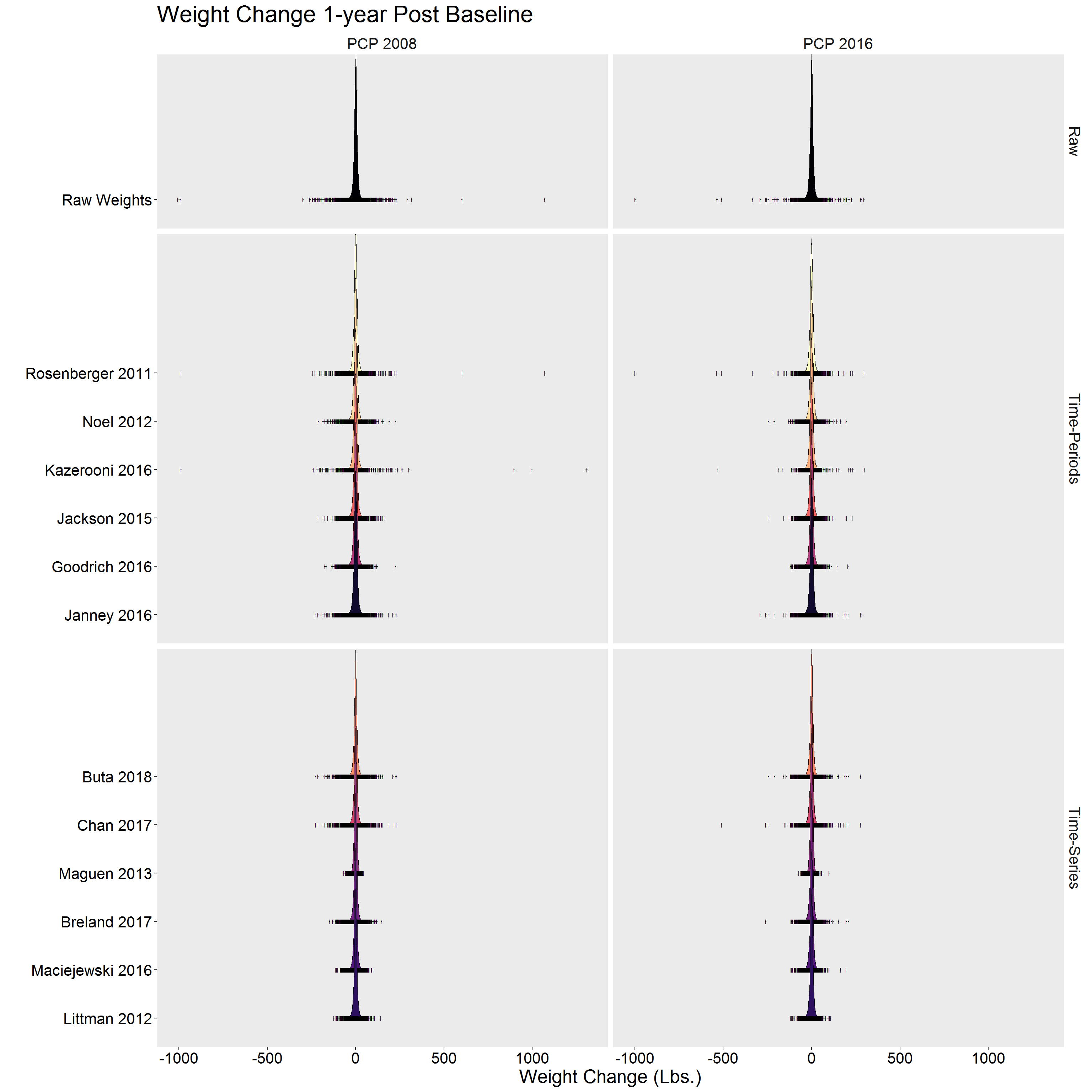
Alternative view
p <- DF %>%
  filter(!is.na(diff)) %>%
  group_by(Algorithm) %>%
  mutate(dens = approxfun(density(diff))(diff)) %>%
  ggplot(aes(y = Algorithm, x = diff, color = dens)) %>%
  add(geom_jitter(size = 2)) %>%
  add(scale_color_viridis_c()) %>%
  add(facet_grid(Type ~ Cohort, scales = "free_y", space = "free_y")) %>%
  add(theme(
    legend.position = "none",
    text = element_text(size = 20),
    axis.text = element_text(color = "black"),
    panel.grid = element_blank(),
    strip.background = element_blank()
  )) %>%
  add(labs(
      x = "Weight Change (Lbs.)",
      y = "",
      title = ""
  ))

p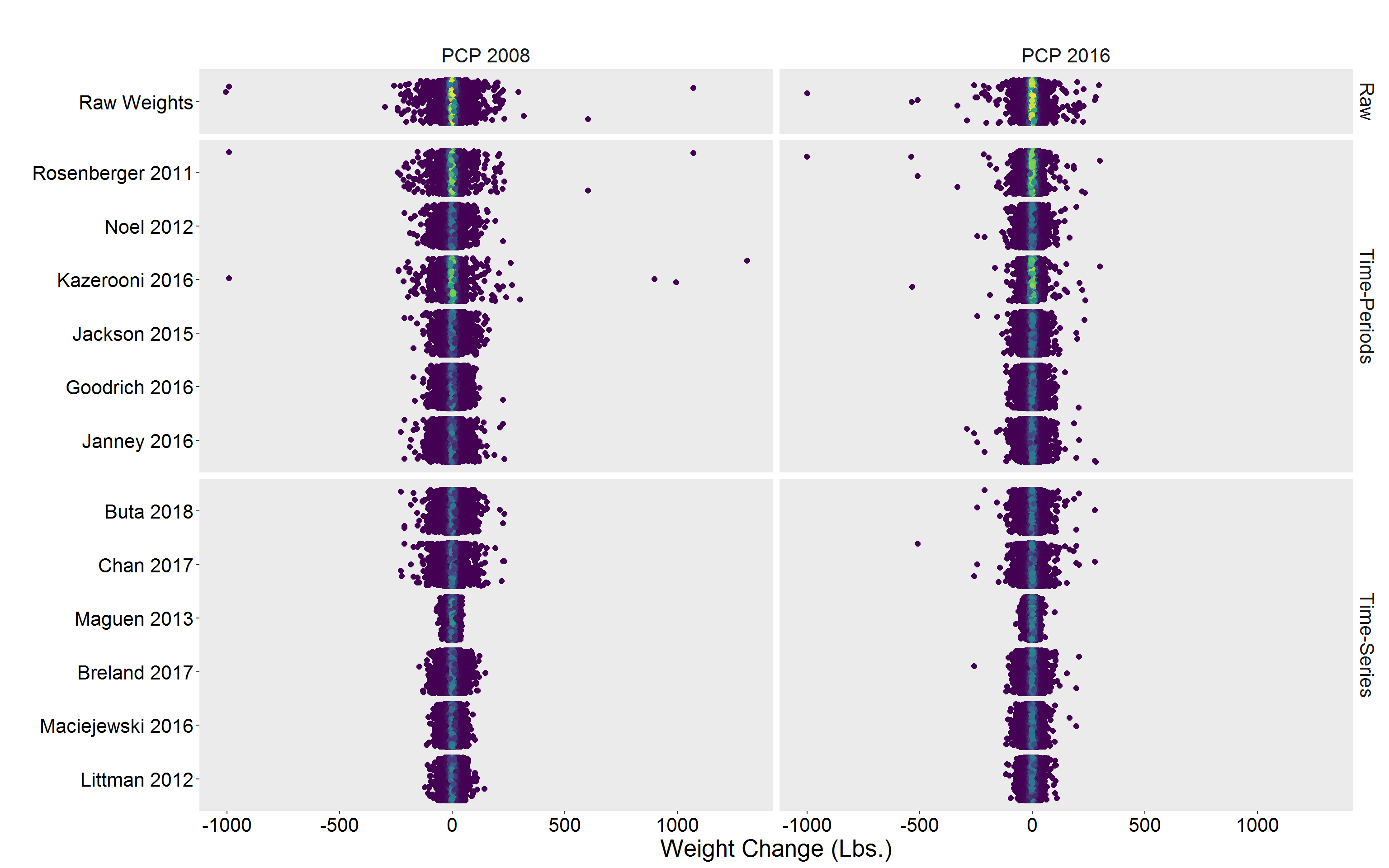
Site/Facility Level
Sta3n_wtdx_diff <- DF %>%
  select(Algorithm, Cohort, Sta3n, diff, diff_perc) %>%
  reshape2::melt(id.vars = c("Cohort", "Algorithm", "Sta3n")) %>%
  group_by(Cohort, Algorithm, Sta3n, variable) %>%
  na.omit() %>%
  summarize(
    n      = n(),
    mean   = mean(value),
    median = median(value)
  ) %>%
  pivot_wider(
    names_from = variable,
    values_from = c("n", "mean", "median")
  )

Sta3n_wtpct <- DF %>%
  select(Cohort, Algorithm, Sta3n, contains("weight")) %>%
  reshape2::melt(id.vars = c("Cohort", "Algorithm", "Sta3n")) %>%
  group_by(Cohort, Algorithm, Sta3n, variable) %>%
  summarize(prop = sum(value == 1) / n()) %>%
  pivot_wider(names_from = variable, values_from = "prop")

Sta3n_wtdx <- Sta3n_wtdx_diff %>%
  left_join(Sta3n_wtpct, by = c("Cohort", "Algorithm", "Sta3n")) %>%
  left_join(
    DF %>%
      distinct(Algorithm, Type),
    by = "Algorithm"
  ) %>%
  select(
    Type,
    Sta3n,
    n_diff,
    mean_diff,
    median_diff,
    mean_diff_perc,
    median_diff_perc,
    gt5perc_weightloss,
    gt5perc_weightgain
  ) %>%
  ungroup()

rm(Sta3n_wtdx_diff, Sta3n_wtpct)

COLS <- c("#2E364F", "#2D5D7C", "#F3F0E2", "#EF5939")

p <- Sta3n_wtdx %>%
  select(Sta3n, mean_diff, median_diff) %>%
  reshape2::melt(id.vars = "Sta3n") %>%
  ggplot(aes(value, group = variable, fill = variable)) %>%
  add(geom_histogram(bins = 40, alpha = 0.5)) %>%
  add(theme_minimal(16)) %>%
  add(theme(legend.position = c(0.2, 0.8))) %>%
  add(scale_fill_manual(values = COLS[c(2, 4)])) %>%
  add(labs(
    x = "Weight Change (lbs.)",
    y = "Frequency",
    fill = ""
  ))

q <- Sta3n_wtdx %>%
  select(Sta3n, mean_diff_perc, median_diff_perc) %>%
  reshape2::melt(id.vars = "Sta3n") %>%
  filter(!is.infinite(value) & value < 1.0) %>%
  ggplot(aes(value, group = variable, fill = variable)) %>%
  add(geom_histogram(bins = 40, alpha = 0.5)) %>%
  add(theme_minimal(16)) %>%
  add(theme(legend.position = c(0.2, 0.8))) %>%
  add(scale_fill_manual(values = COLS[c(2, 4)])) %>%
  add(labs(
    x = "Weight Change %",
    y = "Frequency",
    fill = ""
  ))

r <- Sta3n_wtdx %>%
  ggplot(aes(gt5perc_weightloss)) %>%
  add(geom_histogram(bins = 40, alpha = 0.5, fill = COLS[2])) %>%
  add(theme_minimal(16)) %>%
  add(labs(
    x = ">= 5% Weight Loss",
    y = "Frequency"
  ))

s <- Sta3n_wtdx %>%
  filter(!is.na(gt5perc_weightgain)) %>%
  ggplot(aes(gt5perc_weightgain)) %>%
  add(geom_histogram(bins = 40, alpha = 0.5, fill = COLS[4])) %>%
  add(theme_minimal(16)) %>%
  add(labs(
    x = ">= 5% Weight Gain",
    y = "Frequency"
  ))

library(patchwork)

p + q + r + s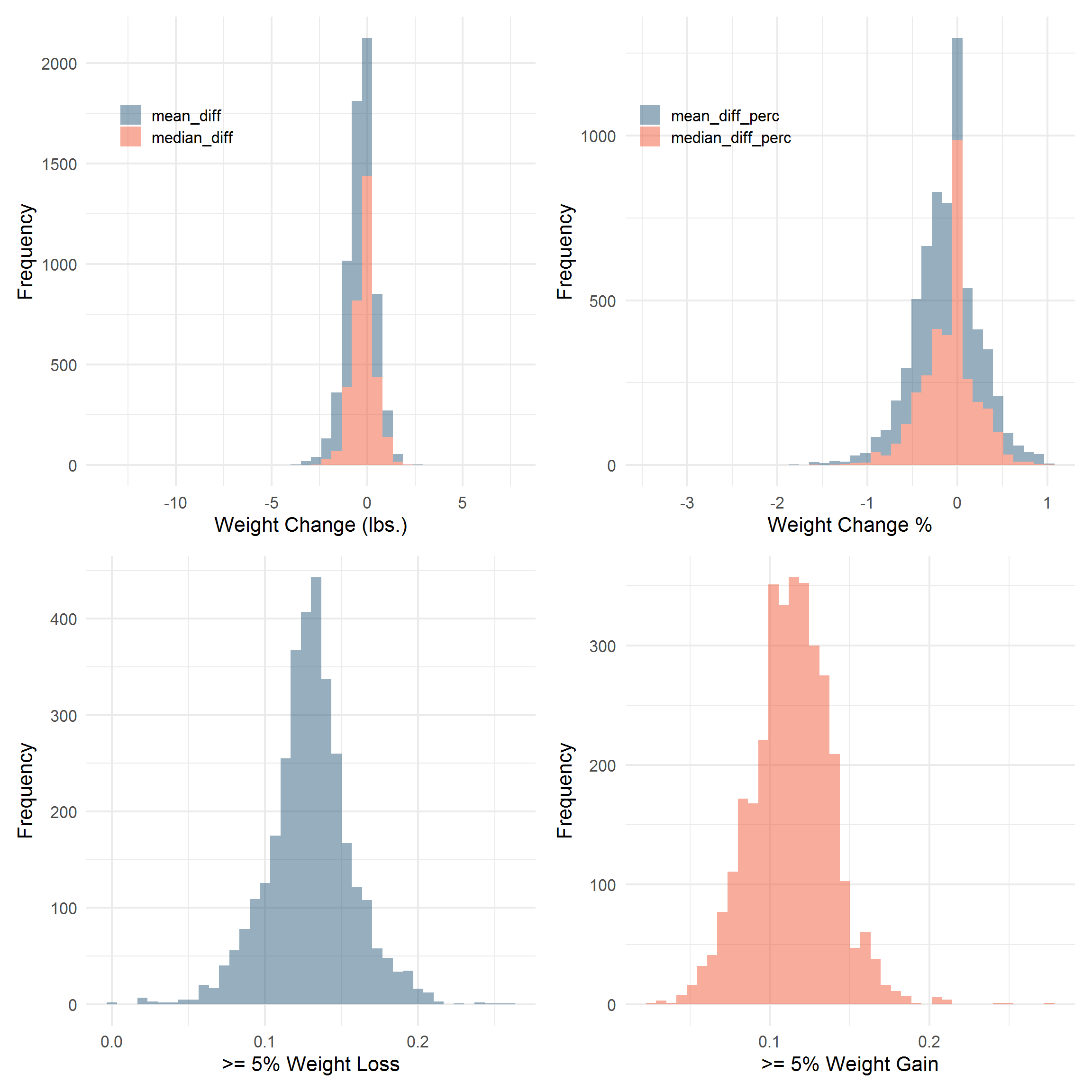
library(gridExtra)

tmp <- Sta3n_wtdx %>%
  filter(Cohort == "PCP 2016") %>%
  select(Type, Algorithm, Sta3n, gt5perc_weightloss)

raw <- tmp %>%
  filter(Algorithm == "Raw Weights") %>%
  arrange(gt5perc_weightloss) %>%
  mutate(Sta3n_rank = row_number()) %>%
  select(-Type, -Algorithm) %>%
  rename(raw_wtloss = gt5perc_weightloss)

tp <- tmp %>%
  filter(Type == "Time-Periods") %>%
  left_join(raw, by = "Sta3n") %>%
  mutate(loss_diff = gt5perc_weightloss - raw_wtloss)

ts <- tmp %>%
  filter(Type == "Time-Series") %>%
  left_join(raw, by = "Sta3n") %>%
  mutate(loss_diff = gt5perc_weightloss - raw_wtloss)

p1 <- tp %>%
  ggplot(aes(x = Sta3n_rank, y = raw_wtloss)) %>%
  add(facet_wrap(vars(Type), ncol = 2)) %>%
  add(geom_line(size = 1)) %>%
  add(geom_segment(
    aes(
      x = Sta3n_rank,
      y = raw_wtloss,
      xend = Sta3n_rank,
      yend = gt5perc_weightloss
    ),
    alpha = 0.3
  )) %>%
  add(geom_point(
    aes(
      x = Sta3n_rank,
      y = gt5perc_weightloss,
      color = Algorithm
    ),
    size = 2,
    alpha = 0.7
  )) %>%
  add(expand_limits(y = c(0.0, 0.3))) %>%
  add(theme_minimal(16)) %>%
  add(theme(
    legend.position = "bottom",
    panel.grid.major.x = element_blank(),
    panel.grid.minor.x = element_blank()
  )) %>%
  add(guides(color = guide_legend(override.aes = list(size = 5)))) %>%
  add(scale_color_brewer(palette = "Dark2")) %>%
  add(labs(
    x = "Sta3n",
    y = "Proportion Achieving 5% Weight Loss",
    color = ""
  ))

p2 <- p1 %+% ts
p2 <- p2 %>% add(labs(y = ""))
grid.arrange(p1, p2, ncol = 2)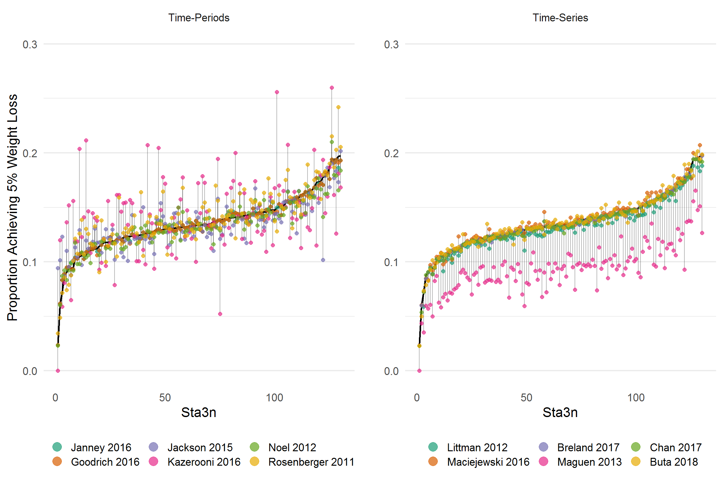
Wyndy Wiitala created this version in STATA:
/*
Algorithm   Freq.   Percent Cum.

1: Raw  129 14.29   14.29
2: Janney 2016  129 14.29   28.57
3: Littman 2012 129 14.29   42.86
4: Breland 2017 129 14.29   57.14
5: Maguen 2013  129 14.29   71.43
6: Goodrich 2016    129 14.29   85.71
7: Chan & Raffa 2017    129 14.29   100.00

Total   903 100.00
*/

cd "X:\Damschroder-NCP PEI\6. Aim 2 Weight Algorithms\CDW Data\data"

use Site_Level_wt5, clear
des
tab Algorithm
tab Algorithm, nolab

bys Algorithm: sum prop
bys Algorithm: sum prop, det
gen group=1 if Algorithm==9 | Algorithm==7 | Algorithm==2 | Algorithm==11 | Algorithm==12 | Algorithm==13
replace group=2 if Algorithm==8 | Algorithm==6 | Algorithm==5 | Algorithm==4 | Algorithm==3 | Algorithm==10

bys group Algorithm: sum prop
bys group Algorithm: sum prop, det

sum prop if Algorithm>1

sort prop

forv i=1/13 {
preserve
keep if Algorithm==`i'
gsort prop
gen rank`i'=_n
gen prop`i'=prop
keep Sta3n rank`i' prop`i'
save rank`i', replace
restore
}

use rank1, clear
merge 1:1 Sta3n using rank2
drop _merge
merge 1:1 Sta3n using rank3
drop _merge
merge 1:1 Sta3n using rank4
drop _merge
merge 1:1 Sta3n using rank5
drop _merge
merge 1:1 Sta3n using rank6
drop _merge
merge 1:1 Sta3n using rank7
drop _merge
merge 1:1 Sta3n using rank8
drop _merge
merge 1:1 Sta3n using rank9
drop _merge
merge 1:1 Sta3n using rank10
drop _merge
merge 1:1 Sta3n using rank11
drop _merge
merge 1:1 Sta3n using rank12
drop _merge
merge 1:1 Sta3n using rank13
drop _merge

egen minrank=rowmin(rank2 rank3 rank4 rank5 rank6 rank7 rank8 rank9 rank10
                    rank11 rank12 rank13)
egen maxrank=rowmax(rank2 rank3 rank4 rank5 rank6 rank7 rank8 rank9 rank10
                    rank11 rank12 rank13)
egen minprop=rowmin(prop2 prop3 prop4 prop5 prop6 prop7 prop8 prop9 prop10
                    prop11 prop12 prop13)
egen maxprop=rowmax(prop2 prop3 prop4 prop5 prop6 prop7 prop8 prop9 prop10
                    prop11 prop12 prop13)

egen minpropg1=rowmin(prop2 prop7 prop9 prop11 prop12 prop13)
egen maxpropg1=rowmax(prop2 prop7 prop9 prop11 prop12 prop13)
egen minpropg2=rowmin(prop3 prop4 prop5 prop6 prop8 prop10)
egen maxpropg2=rowmax(prop3 prop4 prop5 prop6 prop8 prop10)

sum minprop, det
sum maxprop, det

sort rank1
*scatter prop1 rank1, mcolor(gs9) msize(vsmall)
line prop1 rank1, lcolor(gs0) lwidth(medium) ///
    || scatter prop2 rank1 , msymbol(diamond)  msize(vsmall) ///
    || scatter prop3 rank1 , msymbol(diamond)  msize(vsmall) ///
    || scatter prop4 rank1 , msymbol(diamond)  msize(vsmall) ///
    || scatter prop5 rank1 , msymbol(diamond)  msize(vsmall) ///
    || scatter prop6 rank1 , msymbol(diamond)  msize(vsmall) ///
    || scatter prop7 rank1 , msymbol(diamond)  msize(vsmall) ///
    || scatter prop8 rank1 , msymbol(diamond)  msize(vsmall) ///
    || scatter prop9 rank1 , msymbol(diamond)  msize(vsmall) ///
    || scatter prop10 rank1 , msymbol(diamond)  msize(vsmall) ///
    || scatter prop11 rank1 , msymbol(diamond)  msize(vsmall) ///
    || scatter prop12 rank1 , msymbol(diamond)  msize(vsmall) ///
    || scatter prop13 rank1 , msymbol(diamond)  msize(vsmall) ///
    || rcap minprop maxprop rank1 , lcolor(black) msize(vsmall) lwidth(vthin)

line prop1 rank1, lcolor(black) lwidth(medium) ///
    || scatter prop2 rank1 , msymbol(diamond)  msize(vsmall) ///
    || scatter prop7 rank1 , msymbol(diamond)  msize(vsmall) ///
    || scatter prop9 rank1 , msymbol(diamond)  msize(vsmall) ///
    || scatter prop11 rank1 , msymbol(diamond)  msize(vsmall) ///
    || scatter prop12 rank1 , msymbol(diamond)  msize(vsmall) ///
    || scatter prop13 rank1 , msymbol(diamond)  msize(vsmall) ///
    || rcap minpropg1 maxpropg1 rank1 , lcolor(gs13) msize(zero) lwidth(thin)
graph save site_5p_g1.gph, replace

line prop1 rank1, lcolor(black) lwidth(medium) ///
    || scatter prop3 rank1 , msymbol(diamond)  msize(vsmall) ///
    || scatter prop4 rank1 , msymbol(diamond)  msize(vsmall) ///
    || scatter prop5 rank1 , msymbol(diamond)  msize(vsmall) ///
    || scatter prop6 rank1 , msymbol(diamond)  msize(vsmall) ///
    || scatter prop8 rank1 , msymbol(diamond)  msize(vsmall) ///
    || scatter prop10 rank1 , msymbol(diamond)  msize(vsmall) ///
    || rcap minpropg2 maxpropg2 rank1 , lcolor(gs13) msize(zero) lwidth(thin)
graph save site_5p_g2.gph, replace

graph combine  site_5p_g1.gph  ///
               site_5p_g2.gph ///
                  , ycommon graphregion(color(white)) iscale(.5)
graph export "X:\Damschroder-NCP PEI\6. Aim 2 Weight Algorithms\CDW Data\Figures\panel_plot_site5p_102119.pdf", replace


gen diffrank=abs(minrank-maxrank)
sum diffrank, det
gen diffprop=abs(minprop-maxprop)
sum diffprop, det
sort Sta3n
hist diffrank

gen rank2_3=abs(rank2-rank3)
gen rank2_4

line sbpmed0 popyr0, lcolor(gs9) lwidth(medium) ///
    || rcap sbploq0 sbpupq0 popyr0 , lcolor(gs9) lwidth(medthin) msize(vsmall) ///
    || scatter sbpmed0 popyr0 , msymbol(diamond) mcolor(gs9) ///
    || line sbpmed1 popyr1, lcolor(black) lwidth(medium) ///
    || rcap sbploq1 sbpupq1 popyr1 , lcolor(black) msize(vsmall) lwidth(medthin) ///
    || scatter sbpmed1 popyr1 , msymbol(square) mcolor(black) ///
    ,ylabel(110(10)150) yscale(r(.,150)) yscale(r(.,110)) ///
    xline(8, lcolor(gray)) xtitle("Years since Start of Study") ///
    xlabel(3(2)17) legend(label(1 "Standard therapy" 2 "Intensive therapy")) legend(off) ///
    graphregion(color(white)) ytitle("SBP")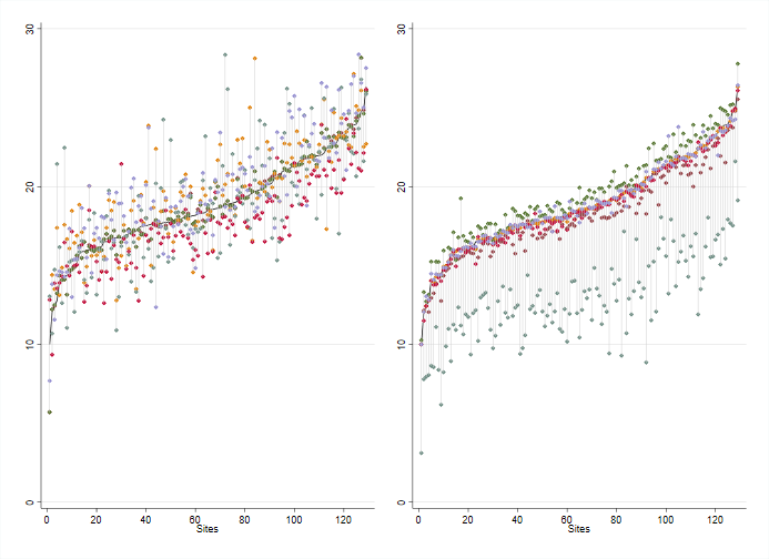
The proportion of individuals acheiving at least 5% weight loss by site.
Sites are ordered/ranked along the x-axis using the percent of patients with at least 5% weight loss using the raw data. The left hand side shows the “time-period” algorithms, while the right displays the “time-series” algorithms. Results suggest that generally, time-series algorithms may result in more similar rates by site, save for Maguen 2013. Results are more mixed using the “time-period” algorithms.