Kazerooni 2016
Excerpt from published methods
Patients were excluded from this study if they were missing weight values from any of the three measuring points of the study (pre-, mid-, and post-weight) … Pre-weight was defined as the most recent weight within 30 days before starting topiramate therapy. Mid-study period was defined as the earliest weight taken between 3 and 6 months post initiation of therapy. Post-study period was defined as the earliest weight taken between 6 and 12 months post initiation of therapy.
Translation in pseudocode
DEFINE time t_ij for person i IN 1:I, j weights In 1:J {pre-trt, mid-trt, post-trt}
FOR i IN 1:I
    FOR j IN 1:J
        weight_i1 := weight @ t_0 (treatment start) - 30 days
        weight_i2 := {t_0 + 90 days <= weight <= t_0 + 180 days}
        weight_i3 := {t_0 + 180 days < weight <= t_0 + 365 days}
    END FOR
    IF (weight_ij IS NULL) (weight measure missing at jth time point)
        EXCLUDE person i
END FOR
Algorithm in R Code
#' @title Kazerooni et al. 2016 Weight Cleaning Algorithm
#' @param DF object of class `data.frame`, containing `id` and `measures`
#' @param id string corresponding to the name of the column of patient identifiers in `DF`
#' @param measures string corresponding to the name of the column of measures in `DF`, e.g., numeric weight data if using to clean weight data.
#' @param tmeasures string corresponding to the name of the column of measure dates and/or times in `DF`
#' @param startPoint string corresponding to the name of the column in `DF` holding the time at which subsequent measurement dates will be assessed, should be the same for each person. Eg., if t = 0 (t[1]) corresponds to an index visit held by the variable 'VisitDate', then `startPoint` should be set to 'VisitDate'
#' @param t numeric vector of time points to collect measurements, eg. `c(0, 182.5, 365)` for measure collection at t = 0, t = 180 (6 months from t = 0), and t = 365 (1 year from t = 0). Default is `c(0, 182.5, 365)` according to Kazerooni et al. 2016
#' @param windows numeric list of two vectors of measurement collection windows to use around each time point in `t`. E.g. Kazerooni et al. 2016 use `c(30, 0, 0)` for the lower bound and `c(0, 0, 185)` for the upper bound at t of `c(0, 90, 180)`, implying that the closest measurement to t[1] (=0) will be within the window [-30, 0], then the closest to t[2] (=90) will be within [90, 180], t[3] (=180) within (180, 365]
Kazerooni2016.f <- function(DF,
                            id,
                            measures,
                            tmeasures,
                            startPoint,
                            t = c(0, 90, 180),
                            windows = list(LB = c(30, 0, 0),
                                           UB = c(0, 90, 185))) {

  if (!require(dplyr)) install.packages("dplyr")
  if (!require(rlang)) install.packages("rlang")

  tryCatch(
    if (class(DF[[tmeasures]])[1] != class(DF[[startPoint]])[1]) {
      stop(
            print(
                  paste0("date type of tmeasures (",
                  class(DF[[tmeasures]]),
                  ") != date type of startPoint (",
                  class(DF[[startPoint]])[1],
                  ")"
                 )
          )
      )
    }
  )

  tryCatch(
    if (class(t) != "numeric") {
      stop(
        print("t parameter must be a numeric vector")
      )
    }
  )

  tryCatch(
    if (!is.list(windows)) {
      stop(
        print("windows must be placed into a list object")
      )
    }
  )

  # compute difference in time between t0 and all t_j
  id         <- rlang::sym(id)
  tmeasures  <- rlang::sym(tmeasures)
  startPoint <- rlang::sym(startPoint)

  DF <- DF %>%
    mutate(
      time = as.numeric(
        difftime(
          !!tmeasures, !!startPoint,
          tz = "utc", units = "days"
        )
      )
    )

  # loop through each time point in `t`, place into list
  meas_tn <- vector("list", length(t)) # set empty list
  for (i in 1:length(t)) {
    meas_tn[[i]] <- DF %>%
      filter(time >= t[i] - windows$LB[i] & time <= t[i] + windows$UB[i]) %>%
      group_by(!!id) %>%
      arrange(abs(time - t[i])) %>%
      slice(1)
  }

  # count number of time points available for each subject i
  do.call(rbind, meas_tn) %>%
    arrange(!!id, !!tmeasures) %>%
    group_by(!!id) %>%
    filter(max(row_number()) >= 3) %>% # must have all 3 time points
    ungroup()
}
Algorithm in SAS Code
Example in R
Kazerooni2016.df <- Kazerooni2016.f(DF,
id = "PatientICN",
measures = "Weight",
tmeasures = "WeightDateTime",
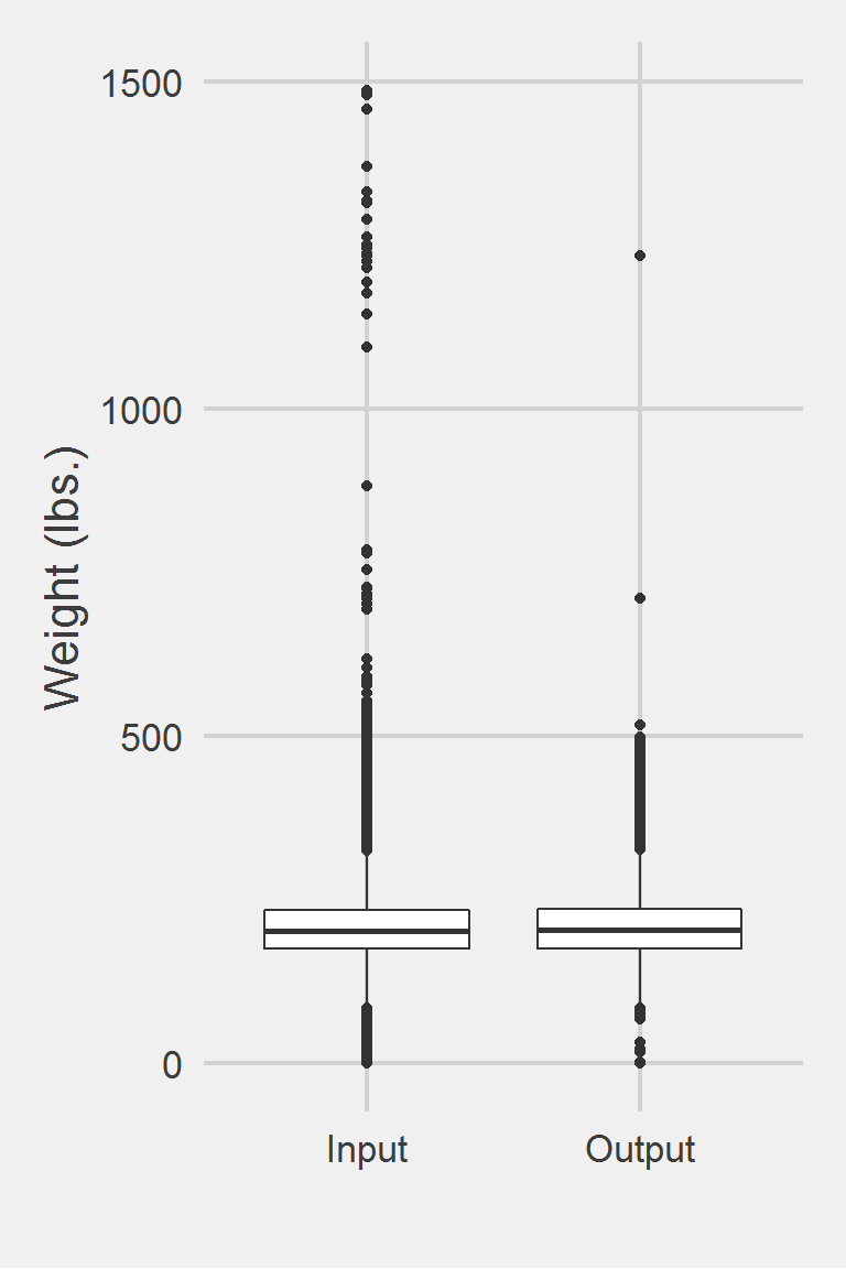
startPoint = "VisitDateTime")Distribution of Weight Measurements between Raw and Algorithm-Processed Values
 Descriptive statistics by group
group: Input
   vars       n   mean   sd median trimmed   mad min    max  range skew
X1    1 1175995 207.82 48.6  202.3  204.62 44.18   0 1486.2 1486.2 0.98
   kurtosis   se
X1      5.6 0.04
------------------------------------------------------------
group: Output
   vars     n mean    sd median trimmed   mad min    max  range skew kurtosis
X1    1 71961  209 47.95    204  206.02 44.33   0 1233.7 1233.7 0.88     4.27
     se
X1 0.18
We won’t show a vignette for Kazerooni & Lim 2016, as it just excludes people, retaining only those with a certain number of measurements.
Left boxplot is raw data from 2016, PCP visit subjects while the right boxplot describes the output from running Kazerooni2016.f()