Rosenberger 2011
Excerpt from published methods
To obtain our study sample, starting from the date of the first VHA healthcare visit for each veteran, we calculated BMI at VHA visits within a six month time frame for up to 6 years. Thus, while all veterans had different actual starting dates, time in the study began for each veteran at their first VHA healthcare visit. Each veteran had at most 12 BMI observations. A missing BMI value was generated if weight was not recorded during a specific 6-month window. We limited our analytic sample to veterans who had at least seven observed BMI values after their last deployment end date. This restriction was necessary to collect sufficient and necessary information for determining the BMI trajectories.
Similar to other studies, Rosenberger et al. based their algorithm on BMI instead of weight, but as usual, the process is the same and proceeding with weight will have no impact on the process. Though, it is important to note that eliminating those without at least 7 BMI values could definitely differ if it is necessary to collect height values at the same time or within a similar time frame, since Rosenberger left this ambiguous, I don’t think it is very important.
Translation in Pseudocode
Algorithm in R Code
#' @title Rosenberger 2011 Measurment Cleaning Algorithm
#' @param DF object of class `data.frame`, containing `id` and `measures`
#' @param id string corresponding to the name of the column of patient identifiers in `DF`
#' @param tmeasures string corresponding to the name of the column of measurement collection dates or times in `DF`. If `tmeasures` is a date object, there may be more than one weight on the same day, if it precise datetime object, there may not be more than one weight on the same day
#' @param startPoint string corresponding to the name of the column in `DF` holding the time at which subsequent measurement dates will be assessed, should be the same for each person. Eg., if t = 0 (t[1]) corresponds to an index visit held by the variable 'VisitDate', then `startPoint` should be set to 'VisitDate'
#' @param t numeric vector of time points to collect measurements, eg. Rosenberger chose a total time period of 6 years, dividing each year into intervals of 6-months each, for a total of 12 time points (`seq(0, 6, 0.5)`).
#' @param pad integer to be appended to `t`. e.g., if set to 1, `t` becomes `t * 365 - 1`, the point is to capture 1 day before t = 0 (t[1]).
#' @param texclude the total number of time points an experimental unit (`id`) must have in order to be included in the final cohort. There is no default, but internally it is set to `floor(length(t) / 2) + 1`.
Rosenberger2011.f <- function(DF,
                              id,
                              tmeasures,
                              startPoint,
                              t = seq(0, 2, by = 0.5),
                              pad = 0,
                              texclude = NULL) {

  if (!require(dplyr))      install.packages("dplyr")
  if (!require(data.table)) install.packages("data.table")
  if (!require(rlang))      install.packages("rlang")

  tryCatch(
    if (class(DF[[tmeasures]])[1] != class(DF[[startPoint]])[1]) {
      stop(
            print(
                  paste0("date type of tmeasures (",
                  class(DF[[tmeasures]]),
                  ") != date type of startPoint (",
                  class(DF[[startPoint]])[1],
                  ")"
                 )
          )
      )
    }
  )

  tryCatch(
    if (class(t) != "numeric") {
      stop(
        print("t parameter must be a numeric vector")
      )
    }
  )

  # convert to data.table
  DT <- data.table::as.data.table(DF)
  setkeyv(DT, id)

  # Step 1: time from startPoint
  DT[,
     time := as.numeric(difftime(get(tmeasures),
                                 get(startPoint),
                                 tz = "UTC",
                                 units = "days"))
     ]

  # Step 2: set time points
  t <- t * 365

  # set pad parameter (within "pad" days)
  t <- t - pad

  # Step 3: split data into intervals defined by t
  DT <- split(DT, cut(DT$time, t, include.lowest = TRUE))

  # select closest measurement to each time point
  DT <- lapply(
    DT,
    function(x) {
      x[order(get(id), time)][, .SD[1], by = id]
    }
  )

  if (is.null(texclude)) {
    texclude <- floor(length(t) / 2) + 1
  }

  id <- rlang::sym(id)
  tmeasures <- rlang::sym(tmeasures)

  # return result
  do.call(rbind, DT) %>%
    arrange(!!id, !!tmeasures) %>%
    group_by(!!id) %>%
    filter(max(row_number()) >= texclude) %>% # must have at least texclude
    ungroup()
}
Algorithm in SAS Code
Example in R
Rosenberger2011.df <- Rosenberger2011.f(DF,
id = "PatientICN",
tmeasures = "WeightDateTime",
startPoint = "VisitDateTime",
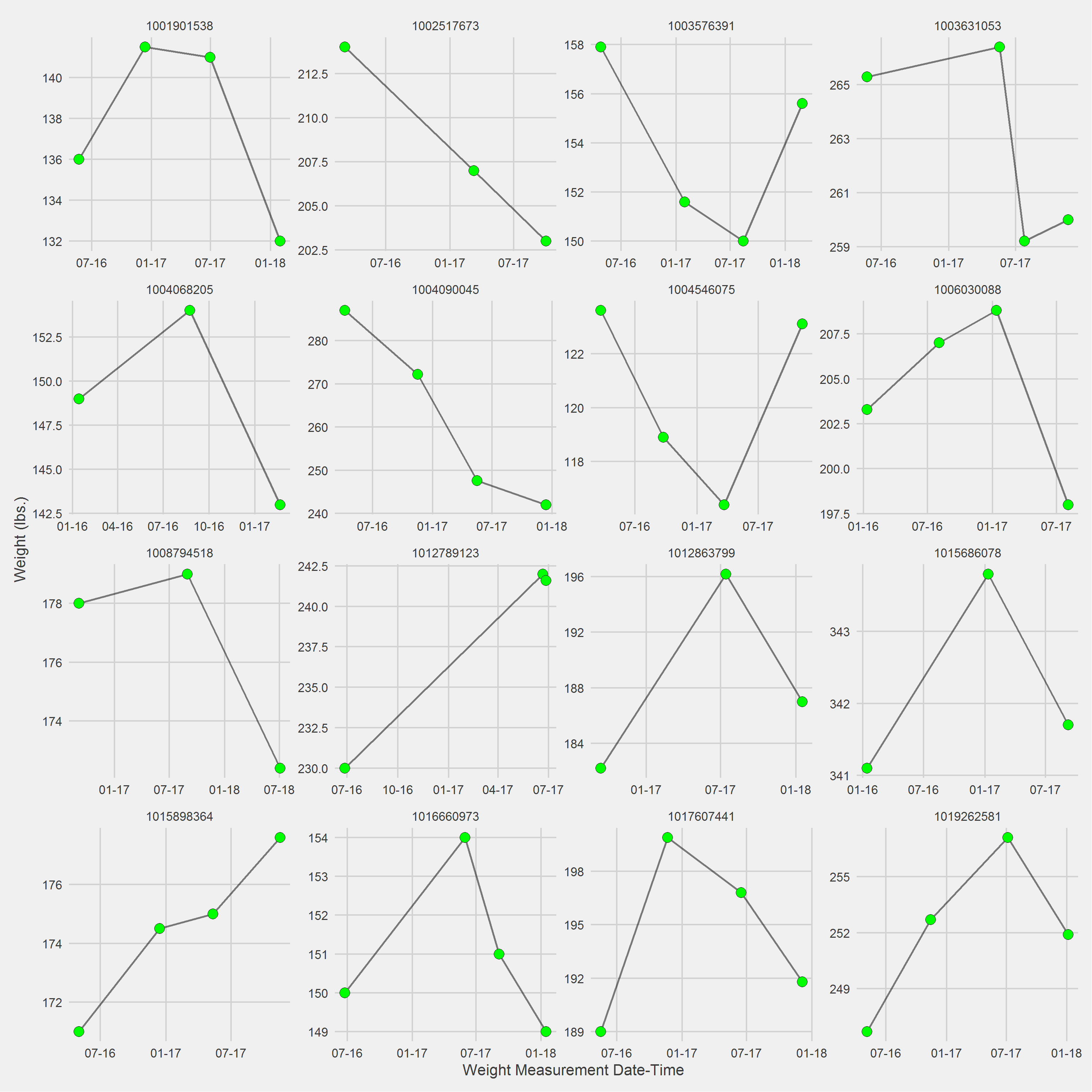
pad = 1)Vignette of 16 randomly selected individuals, displaying weight trajectories since first MOVE! visit in 2016
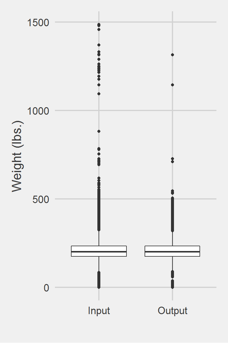
Distribution of Weight Measurements between Raw and Algorithm-Processed Values
 Descriptive statistics by group
group: Input
   vars       n   mean   sd median trimmed   mad min    max  range skew
X1    1 1175995 207.82 48.6  202.3  204.62 44.18   0 1486.2 1486.2 0.98
   kurtosis   se
X1      5.6 0.04
------------------------------------------------------------
group: Output
   vars      n  mean    sd median trimmed   mad min    max  range skew kurtosis
X1    1 227215 207.8 46.23  202.9  204.83 42.25   0 1314.5 1314.5 0.88     3.69
    se
X1 0.1
Left boxplot is raw data from 2016, PCP visit subjects while the right boxplot describes the output from running Rosenberger2011.f()