Poisson Processes

Simulate sample path: fixed number of events

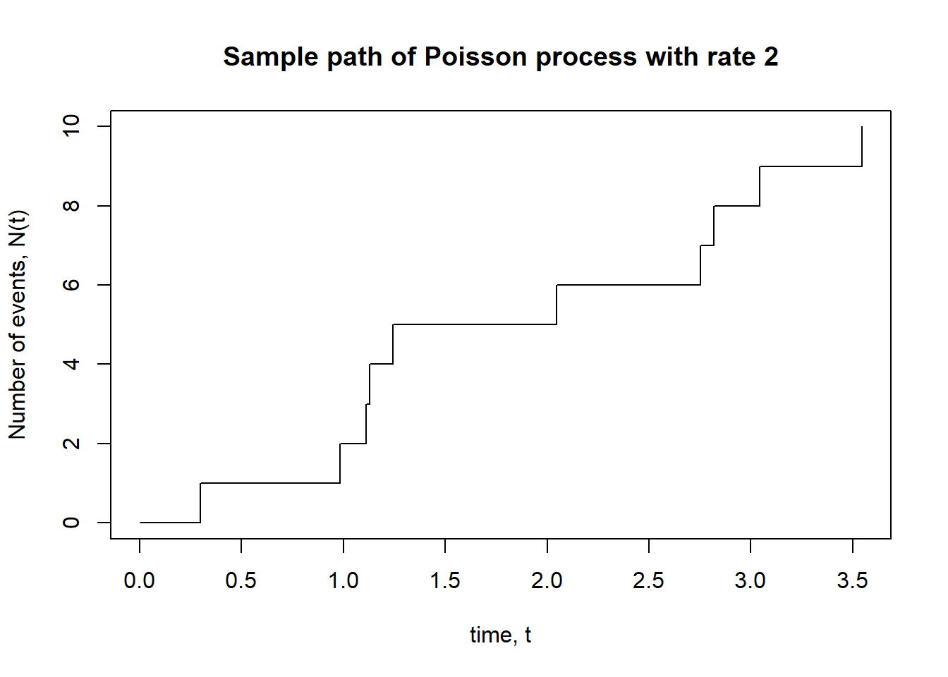
Simulate times between events as i.i.d. Exponential

n = 10

lambda = 2

w = rexp(n, rate = lambda)

t = cumsum(c(0, w))

plot(t, 0:n,
     type = "s",
     xlab = "time, t", ylab = "Number of events, N(t)",
     main = paste("Sample path of Poisson process with rate", lambda))

Simulate sample path: fixed time

Simulate total number of events as Poisson(\(\lambda T\))
Given number of events, simulate times of events as i.i.d. Uniform(0, \(T\)), sorted from smallest to largest

T = 10

lambda = 2

N_T = rpois(1, lambda * T)

u = runif(N_T, 0, T)

t = c(0, sort(u))

plot(t, 0:N_T,
     type = "s",
     xlab = "time, t", ylab = "Number of events, N(t)",
     main = paste("Sample path of Poisson process with rate", lambda))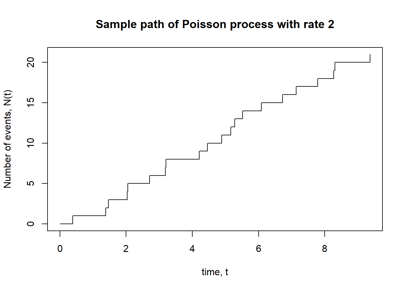

Many sample paths

from symbulate import *

from matplotlib import pyplot as plt

P = PoissonProcessProbabilitySpace(rate = 2)

N = RV(P)

plt.figure()
N.sim(5).plot()
plt.show();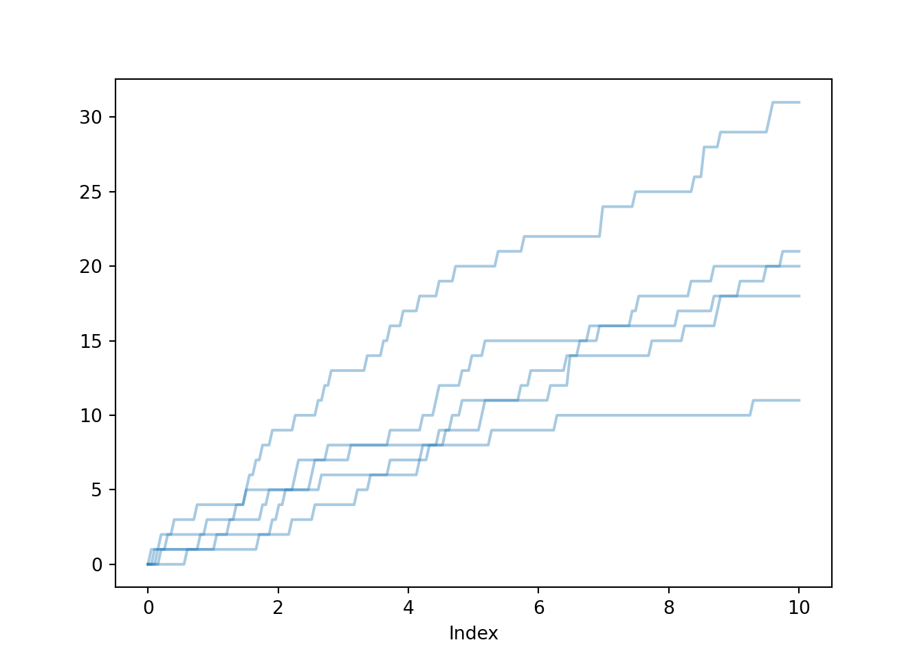

plt.figure()
N.sim(100).plot()
plt.show();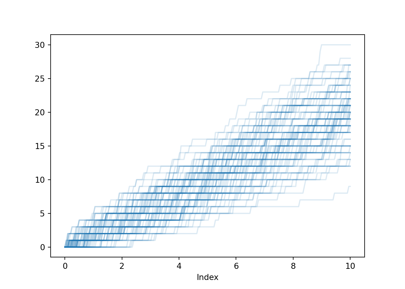

Distribution of process values

plt.figure();

N[5].sim(10000).plot()
Poisson(2 * 5).plot()

<symbulate.distributions.Poisson object at 0x0000017B651B2E50>

plt.show()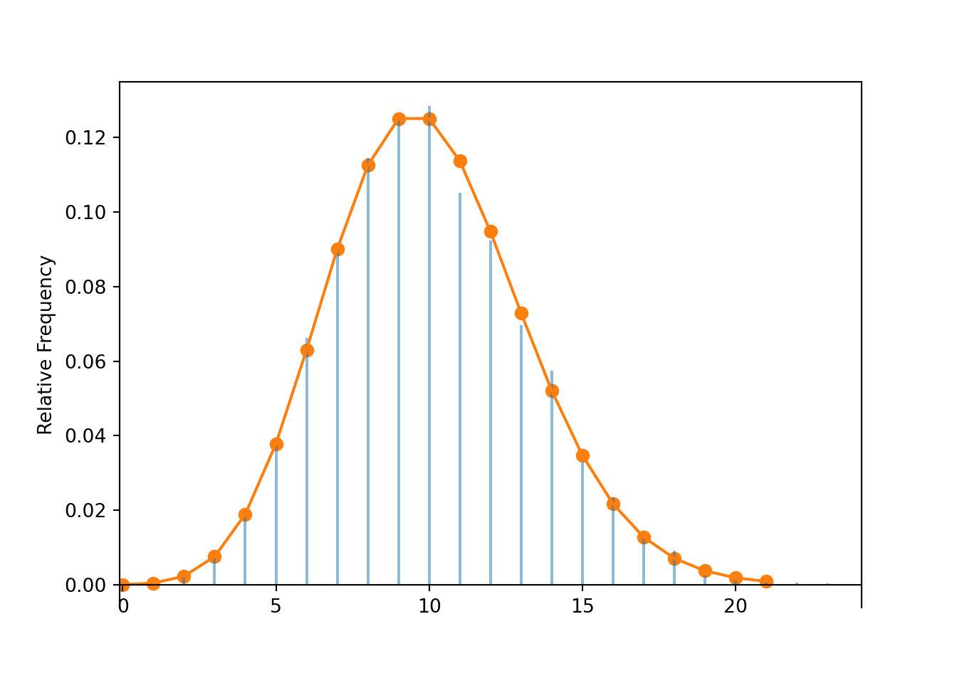

plt.figure();

(N[5] - N[3]).sim(10000).plot()
Poisson(2 * (5 - 3)).plot()

<symbulate.distributions.Poisson object at 0x0000017B65293850>

plt.show()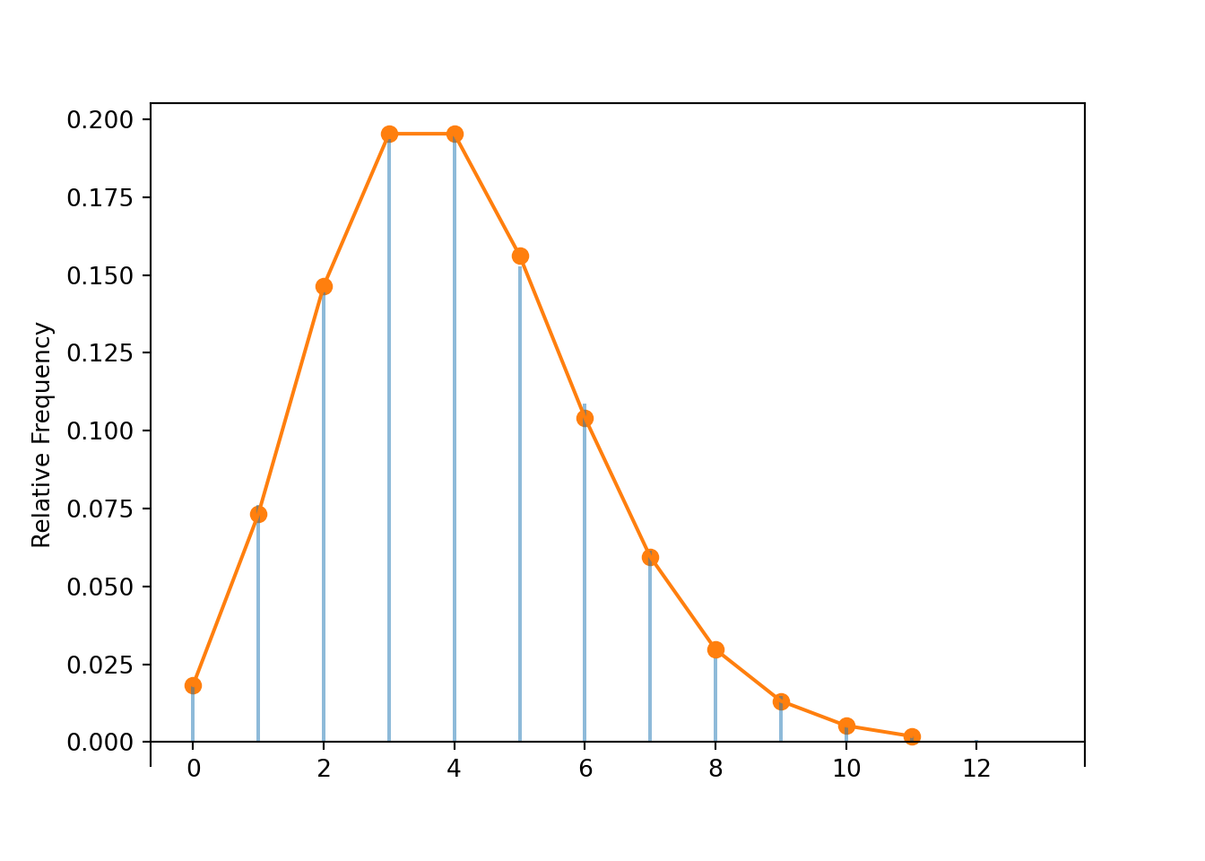

Times between events

W = RV(P, interarrival_times)

plt.figure();
W[0].sim(10000).plot()
Exponential(rate = 2).plot()

<symbulate.distributions.Exponential object at 0x0000017B6549BA10>

plt.show();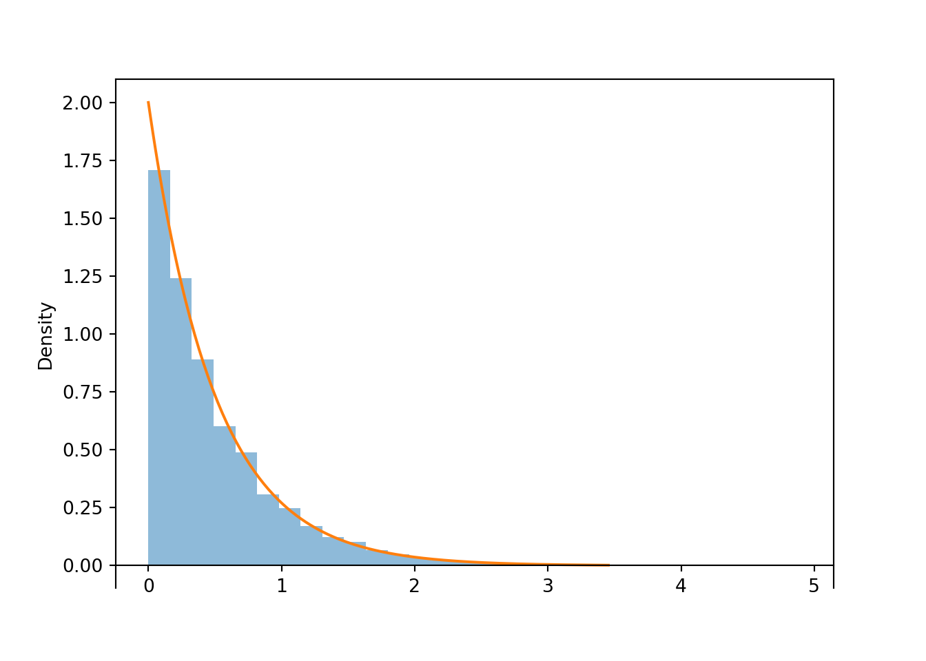

plt.figure();
(W[0] & W[1]).sim(10000).plot()
plt.show();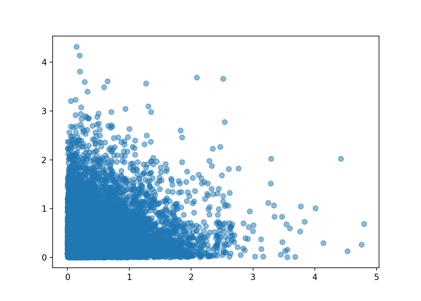

Times of events

T = RV(P, arrival_times)

plt.figure();
T[0].sim(10000).plot()
Gamma(shape = 1, rate = 2).plot()

<symbulate.distributions.Gamma object at 0x0000017B64300410>

plt.show();

plt.figure();
T[1].sim(10000).plot()
Gamma(shape = 2, rate = 2).plot()

<symbulate.distributions.Gamma object at 0x0000017B642467D0>

plt.show();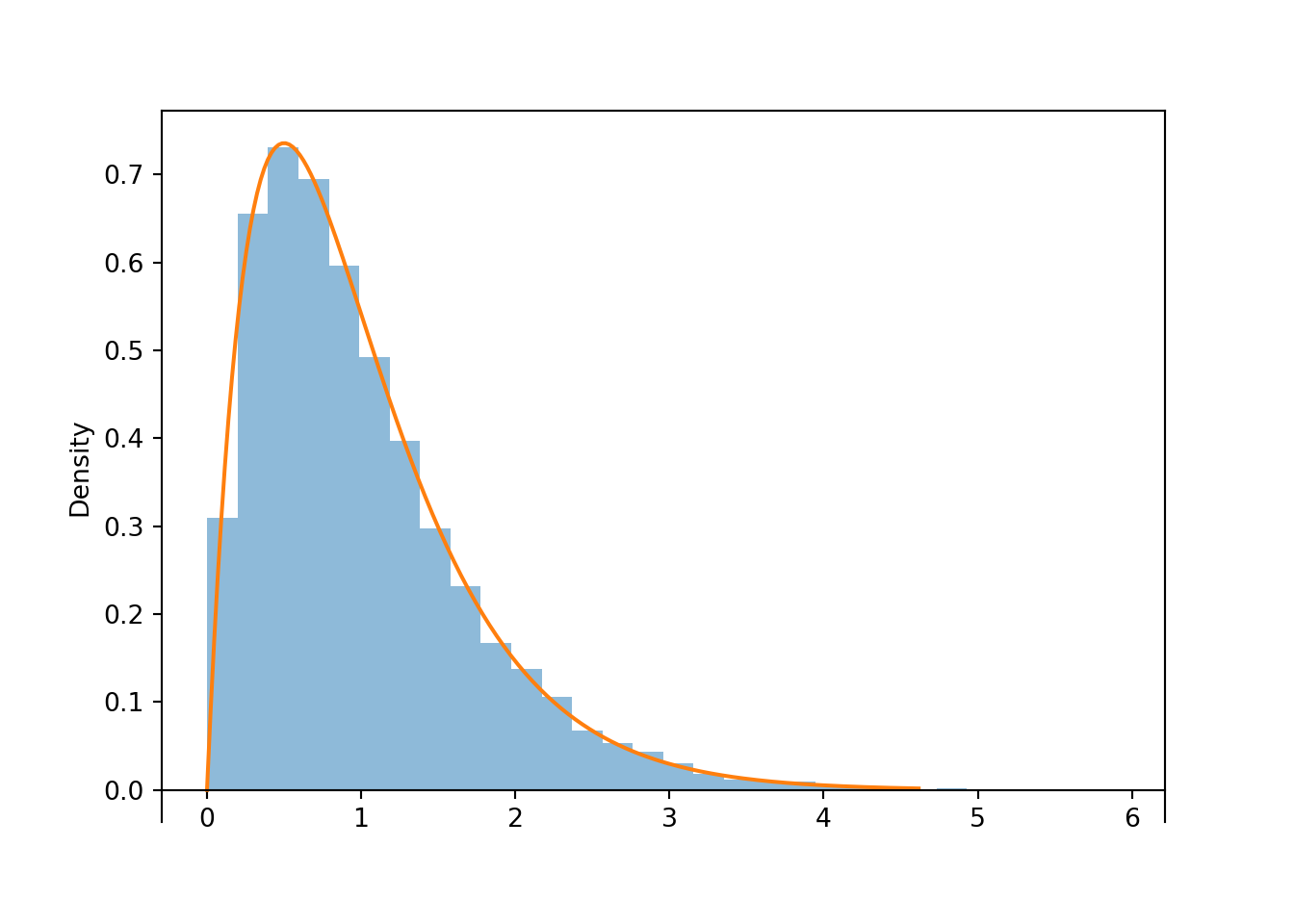

Short time interval

plt.figure();
N[0.05].sim(10000).plot()
plt.show();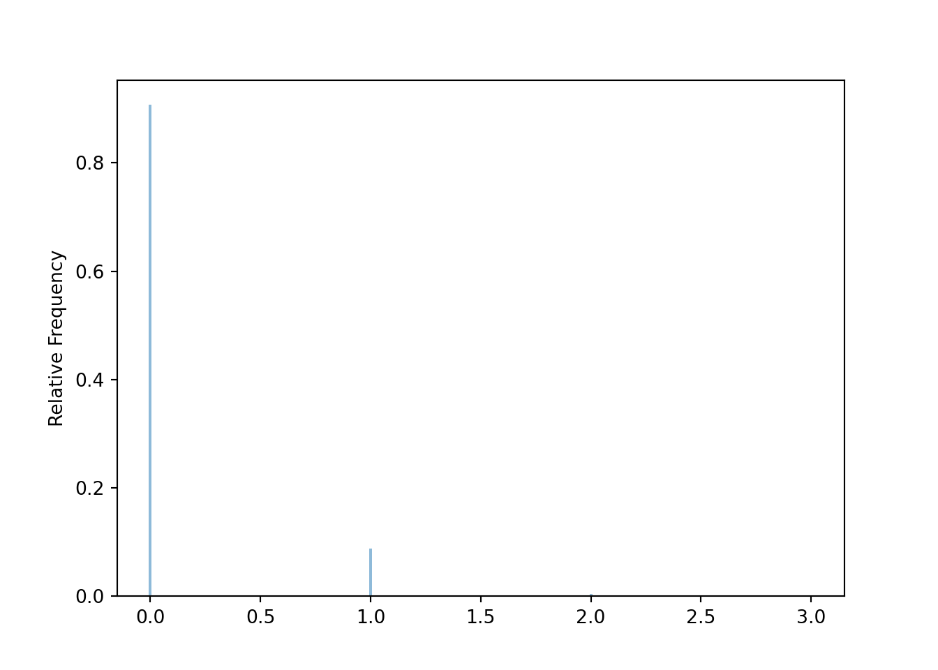

Conditional distribution

plt.figure();
(N[2] | (N[5] == 10) ).sim(10000).plot()
Binomial(10, 2 / 5).plot()

<symbulate.distributions.Binomial object at 0x0000017B63D13910>

plt.show();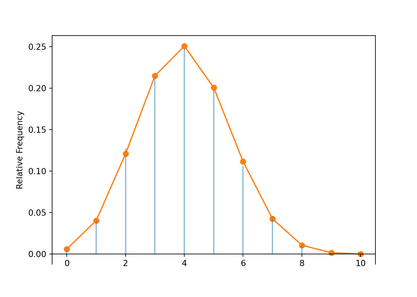

Conditional distribution of arrival times

plt.figure();
(T[0] | (N[2] == 1) ).sim(10000).plot()
Uniform(0, 2).plot()

<symbulate.distributions.Uniform object at 0x0000017B64302E50>

plt.show();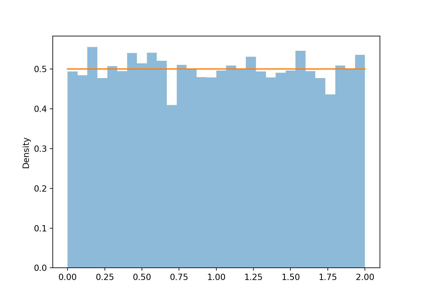

plt.figure();
((T[0] & T[1]) | (N[2] == 2) ).sim(1000).plot()
plt.show();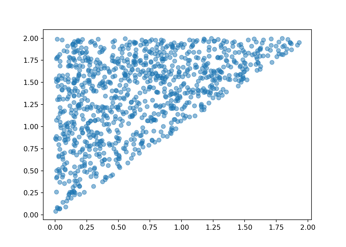

Order statistics of Uniform

plt.figure();
P = Uniform(0, 2) ** 2
U1 = RV(P, min)
U2 = RV(P, max)
(U1 & U2).sim(1000).plot()
plt.show();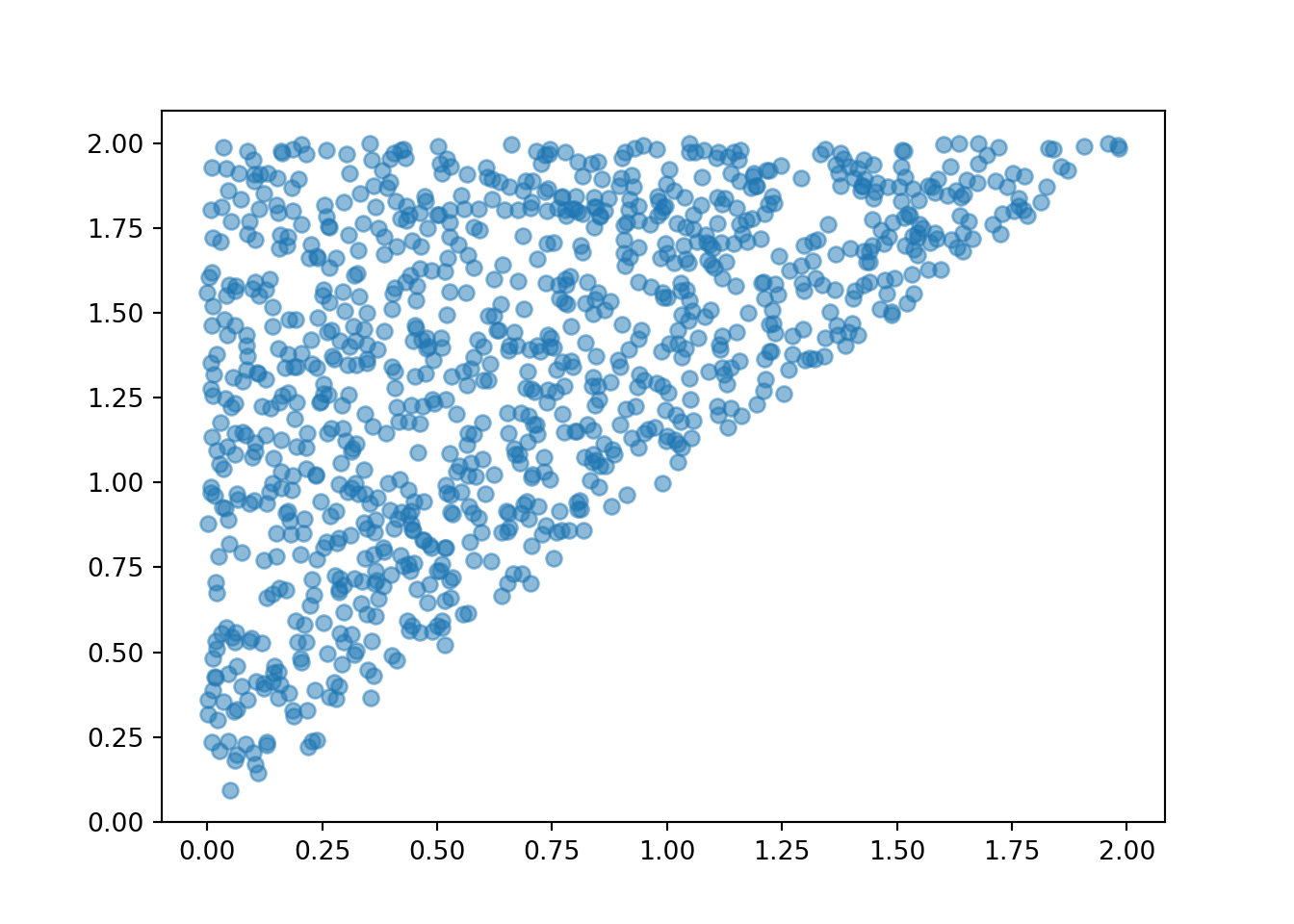

Waiting time paradox

Tmax = 10000
T = 5 #mean time between buses
lambda = 2

N_commuters = rpois(1, lambda * Tmax)
W_commuters = sort(runif(N_commuters, 0 , Tmax))
N_buses = rpois(1, Tmax / T)
W_buses = sort(runif(N_buses, 0 , Tmax))

waiting_time = rep(NA, N_commuters)
for (i in 1:N_commuters){
  if (W_commuters[i] < max(W_buses)){
    waiting_time[i] = min(W_buses[W_buses > W_commuters[i]]) - W_commuters[i]
  }
}
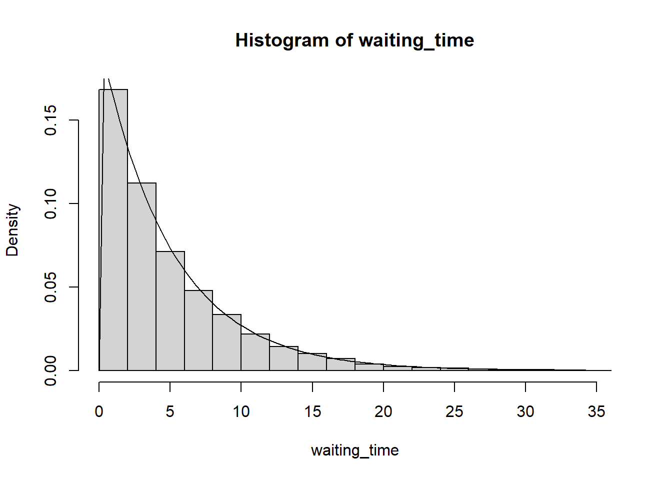
mean(waiting_time, na.rm = TRUE)

[1] 4.908867

hist(waiting_time, freq = FALSE)
curve(dexp(x, 1 / T), add = TRUE)