state_names = c("ice cream", "popcorn")

P = rbind(
  c(0.2, 0.8),
  c(0.4, 0.6)
)Markov Chains: Joint, Conditional, and Marginal Distributions
Popcorn and ice cream
Transition matrix
plot_transition_matrix(P, state_names)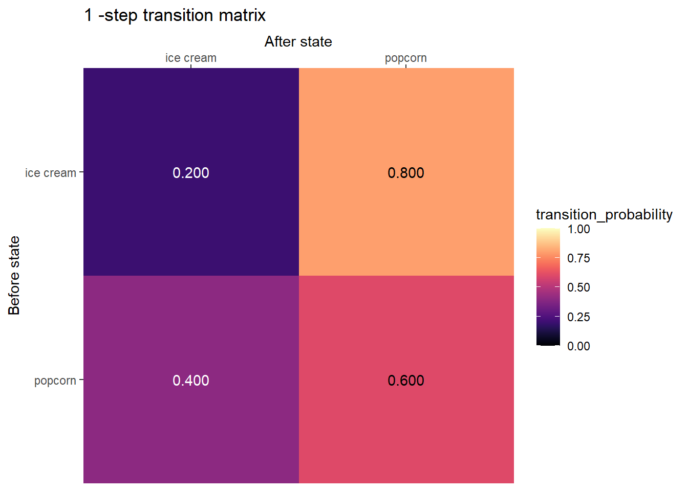
2-step transition matrix
P %*% P [,1] [,2]
[1,] 0.36 0.64
[2,] 0.32 0.68library(expm)
P %^% 2 [,1] [,2]
[1,] 0.36 0.64
[2,] 0.32 0.68plot_transition_matrix(P, n_step = 2)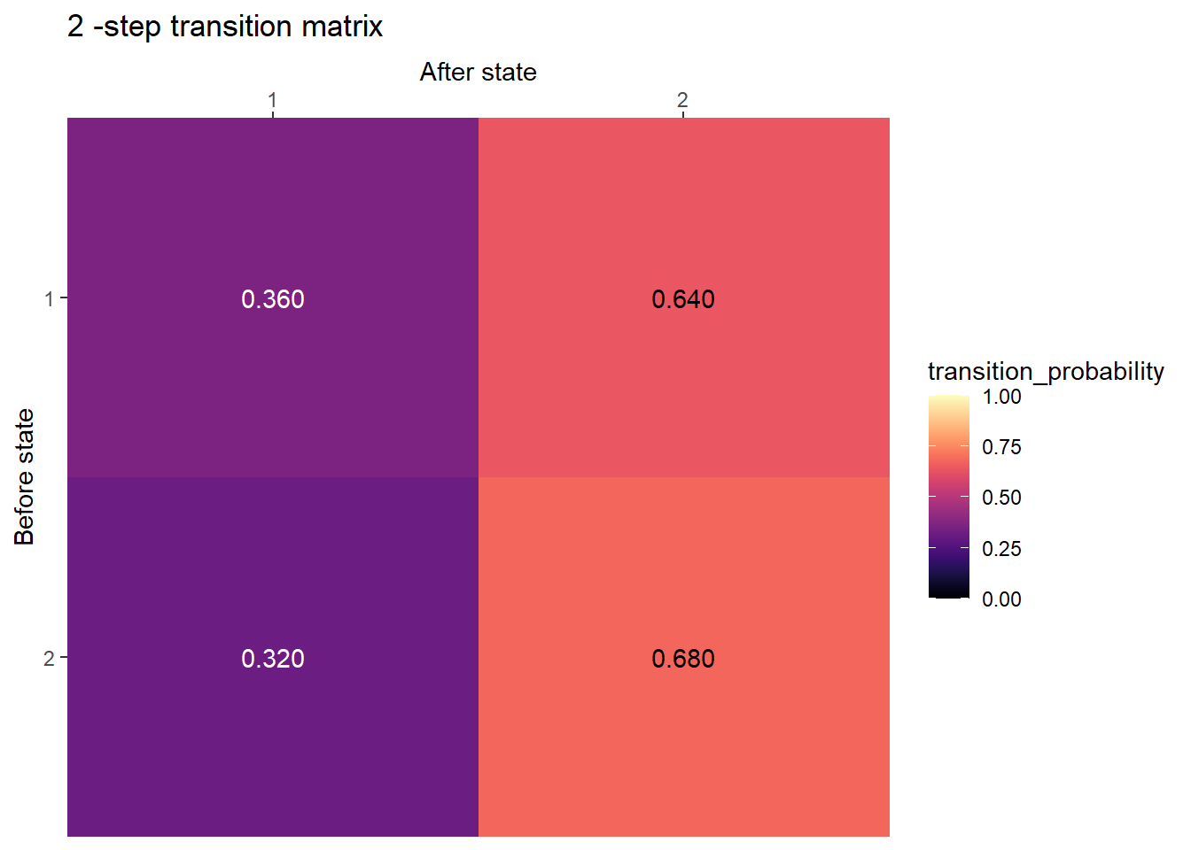
3-step transition matrix
P %^% 3 [,1] [,2]
[1,] 0.328 0.672
[2,] 0.336 0.664plot_transition_matrix(P, n_step = 3)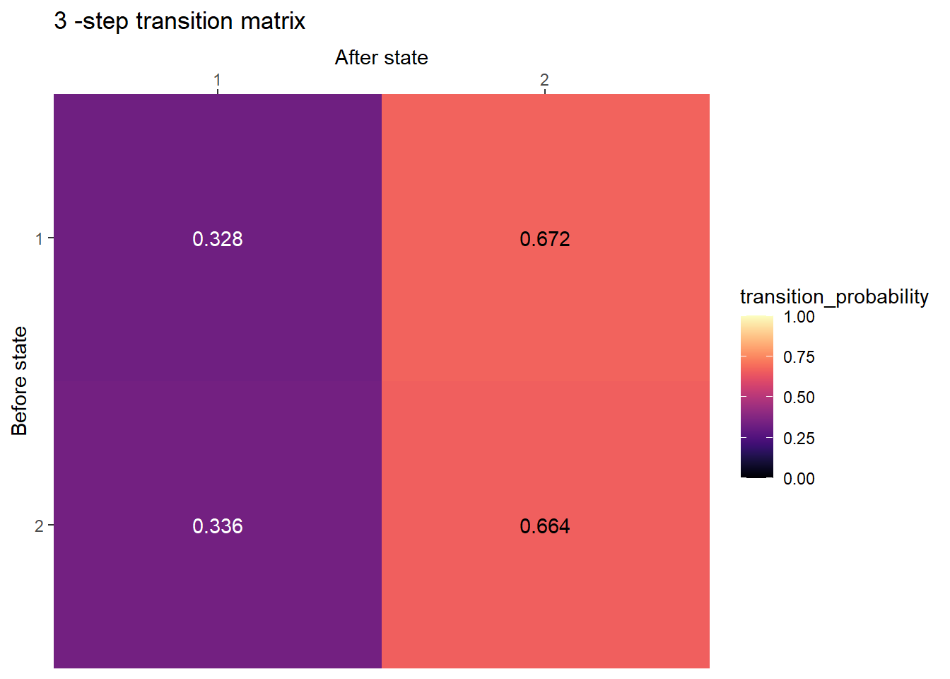
Weather chain
state_names = c("RR", "NR", "RN", "NN")

P = rbind(c(.7, 0, .3, 0),
          c(.5, 0, .5, 0),
          c(0, .4, 0, .6),
          c(0, .2, 0, .8)
)
Transition matrix
plot_transition_matrix(P, state_names)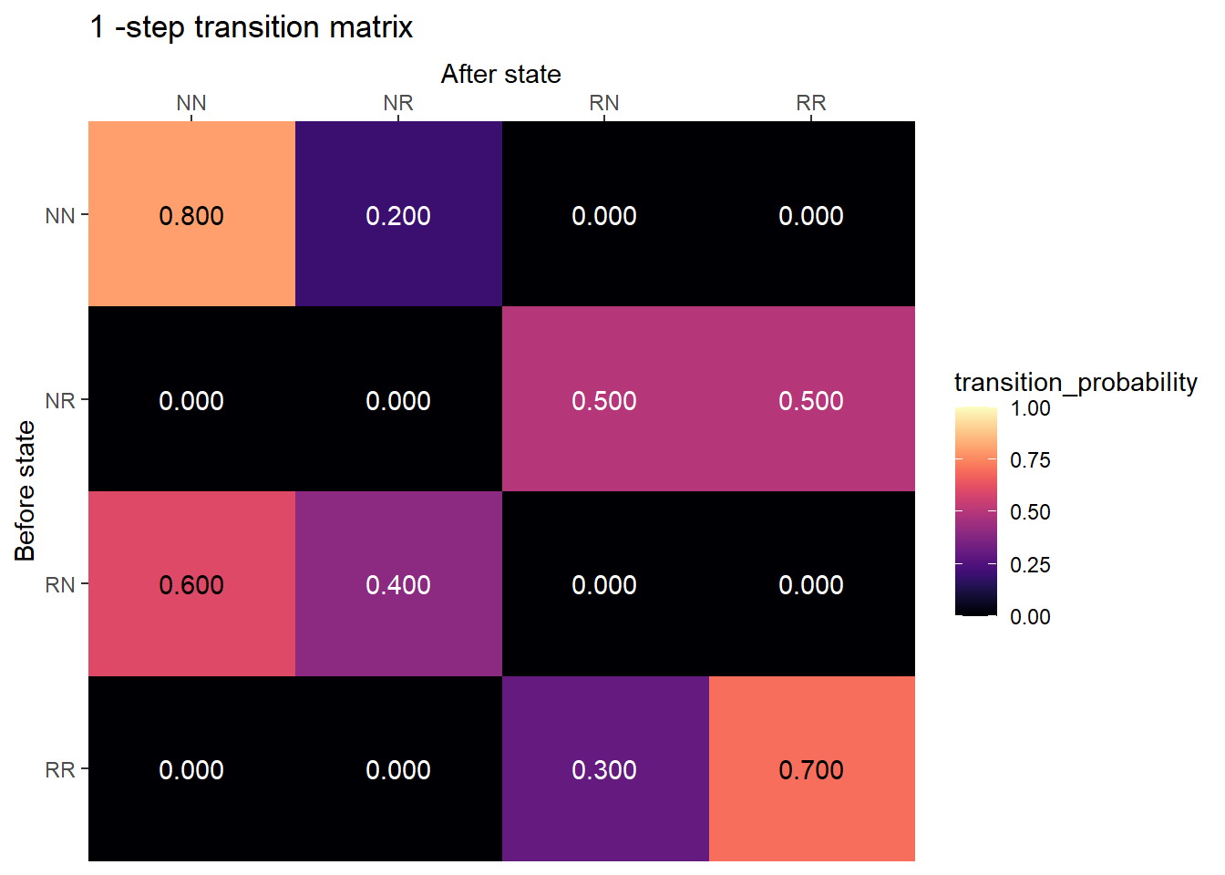
2-step transition matrix
plot_transition_matrix(P, state_names, n_step = 2)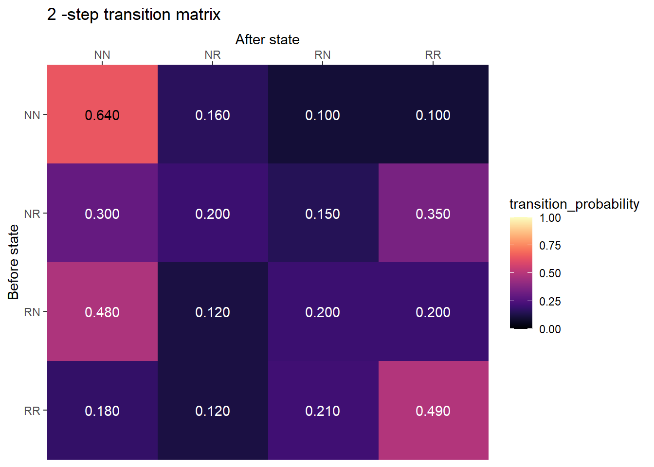
2-step transition matrix
plot_transition_matrix(P, state_names, n_step = 3)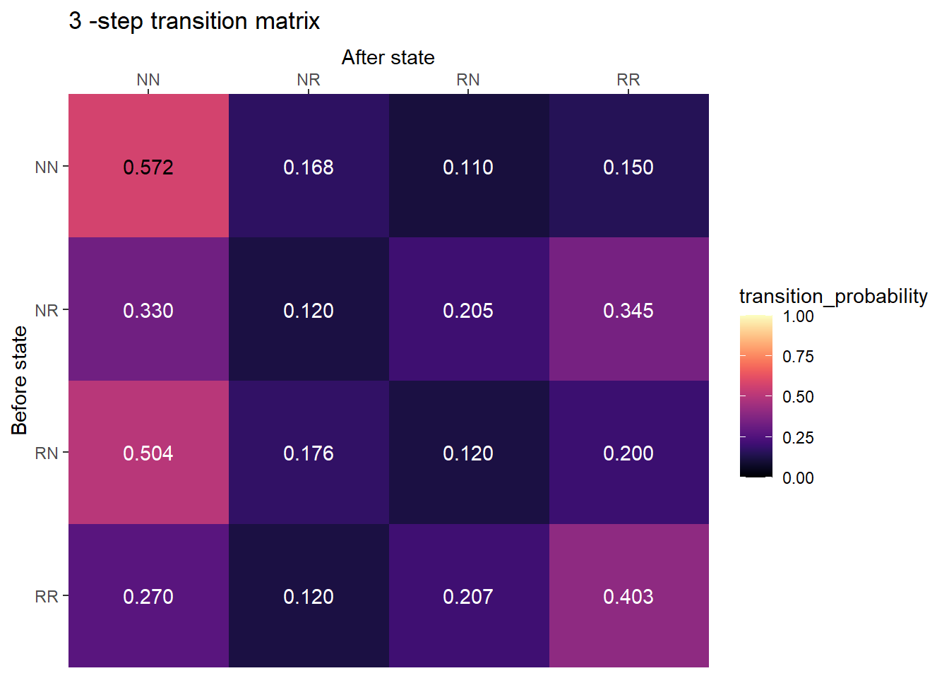
Ping pong
state_names = c("AB", "AC", "BC")

P = rbind(c(0, .7, .3),
          c(.8, 0, .2),
          c(.6, .4, 0)
)
Initial players chosen at random
pi_0 = c(1/3, 1/3, 1/3)

pi_0 %*% P
[,1] [,2] [,3]
[1,] 0.4666667 0.3666667 0.1666667plot_DTMC_marginal_bars(pi_0, P, state_names, last_time = 10)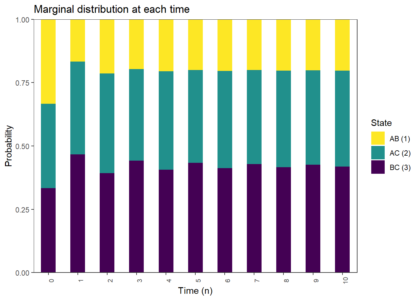
Player A’s initial opponent chosen at random
pi_0 = c(1/2, 1/2, 0)

pi_0 %*% P
[,1] [,2] [,3]
[1,] 0.4 0.35 0.25plot_DTMC_marginal_bars(pi_0, P, state_names, last_time = 10)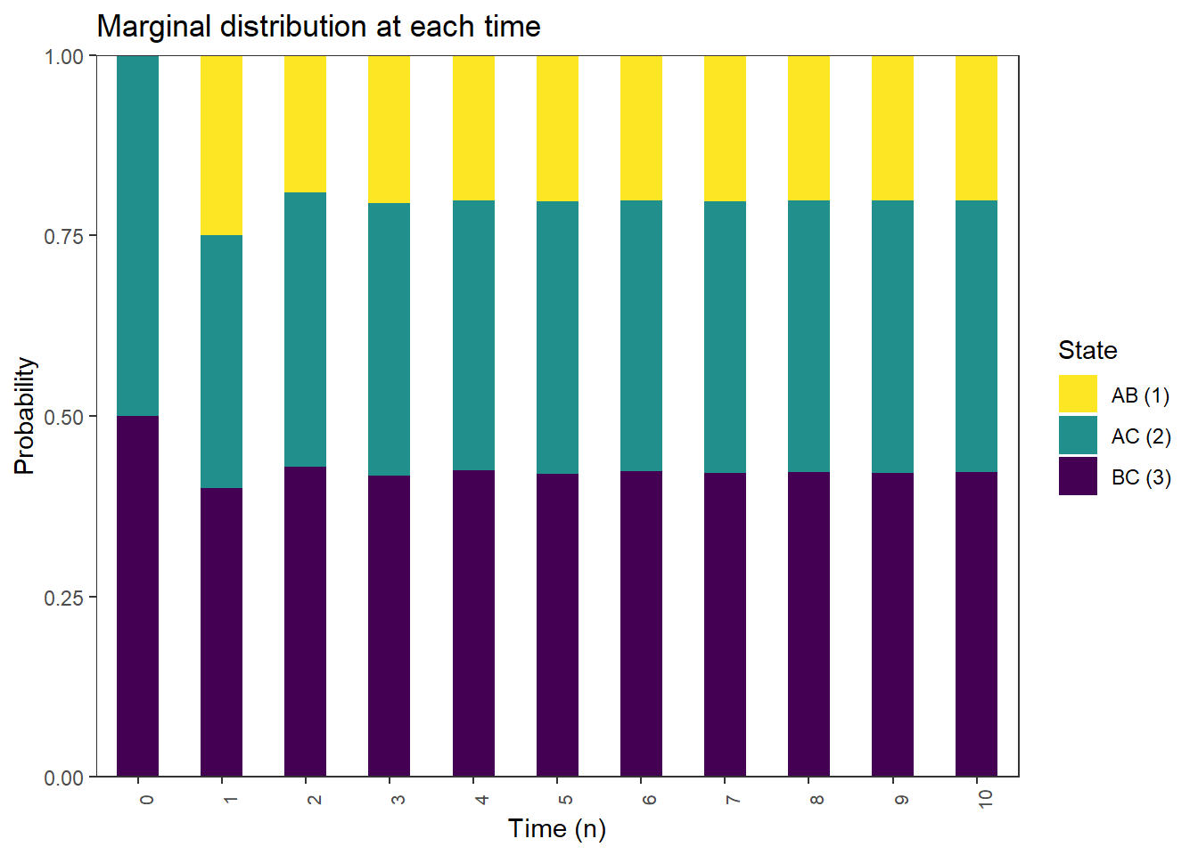
Player A and B play initially
pi_0 = c(1, 0, 0)

pi_0 %*% P
[,1] [,2] [,3]
[1,] 0 0.7 0.3plot_DTMC_marginal_bars(pi_0, P, state_names, last_time = 10)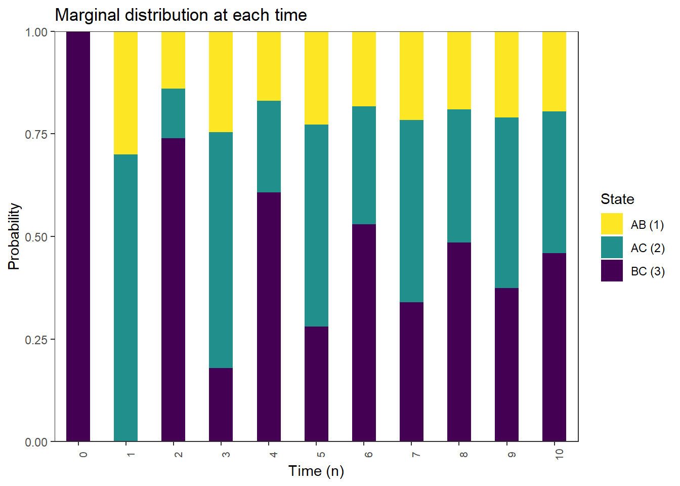
Ehrenfest urn chain
M = 3

state_names = 0:M

P = rbind(c(0, 1, 0, 0),
         c(1/3, 0, 2/3, 0),
         c(0, 2/3, 0, 1/3),
         c(0, 0, 1, 0)
)
Molecules initially distributed at random between A and B
Marginal distribution of \(X_0\)
pi_0 = dbinom(0:M, M, 0.5)

pi_0
[1] 0.125 0.375 0.375 0.125Marginal distribution of \(X_1\)
pi_0 %*% P [,1] [,2] [,3] [,4]
[1,] 0.125 0.375 0.375 0.125Marginal distribution of \(X_2\)
pi_0 %*% (P %^% 2) [,1] [,2] [,3] [,4]
[1,] 0.125 0.375 0.375 0.125Marginal distribution of \(X_3\)
pi_0 %*% (P %^% 3) [,1] [,2] [,3] [,4]
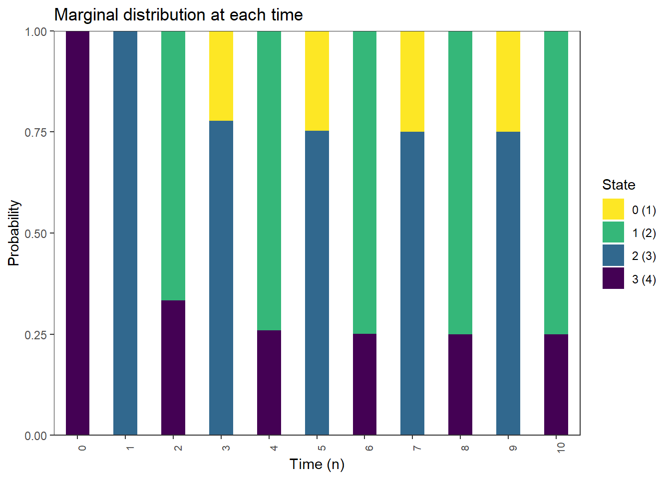
[1,] 0.125 0.375 0.375 0.125plot_DTMC_marginal_bars(pi_0, P, state_names, last_time = 10)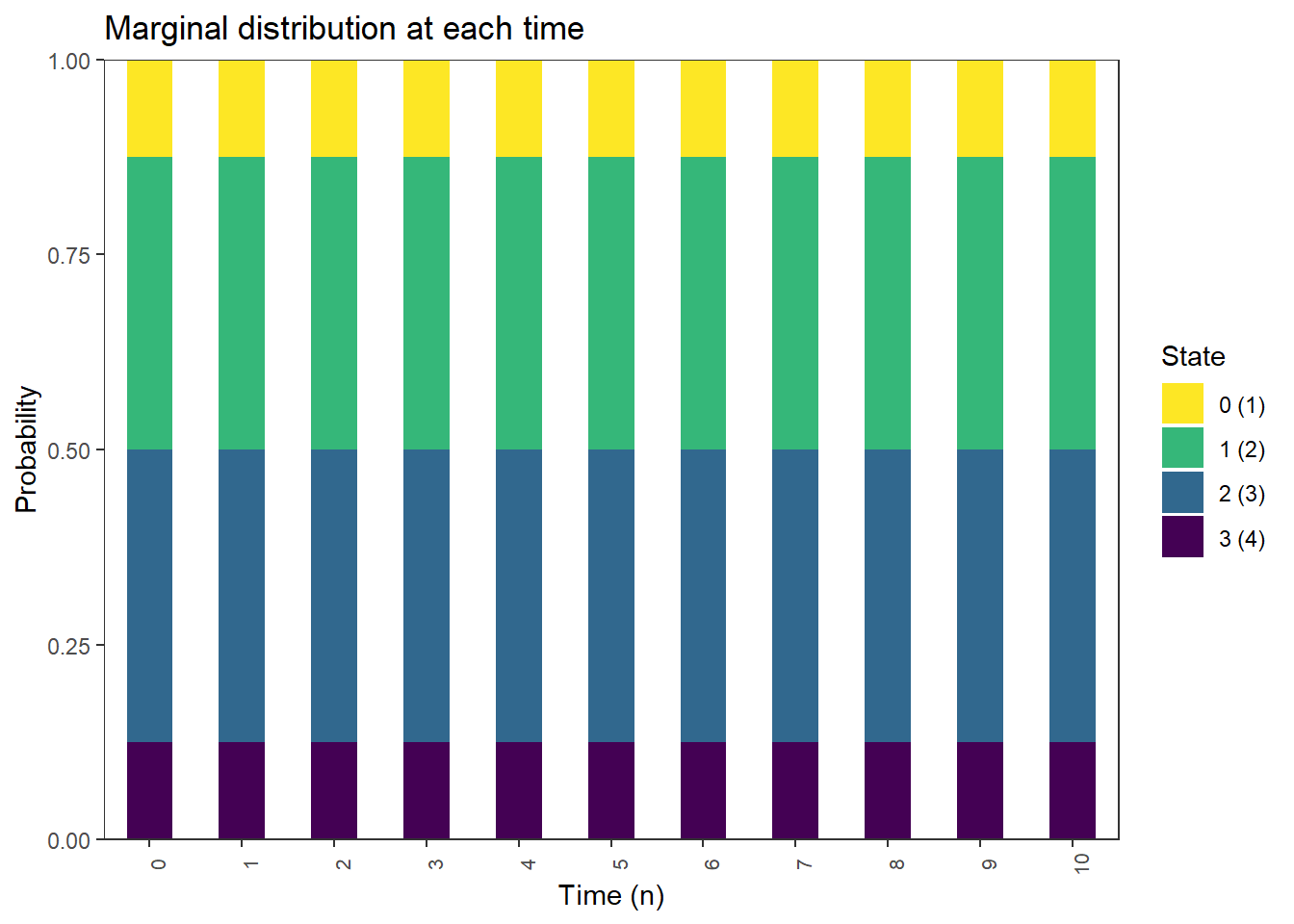
Molecules initially all in A
Marginal distribution of \(X_0\)
pi_0 = c(rep(0, M), 1)

pi_0
[1] 0 0 0 1Marginal distribution of \(X_1\)
pi_0 %*% P [,1] [,2] [,3] [,4]
[1,] 0 0 1 0Marginal distribution of \(X_2\)
pi_0 %*% (P %^% 2) [,1] [,2] [,3] [,4]
[1,] 0 0.6666667 0 0.3333333Marginal distribution of \(X_3\)
pi_0 %*% (P %^% 3) [,1] [,2] [,3] [,4]
[1,] 0.2222222 0 0.7777778 0plot_DTMC_marginal_bars(pi_0, P, state_names, last_time = 10)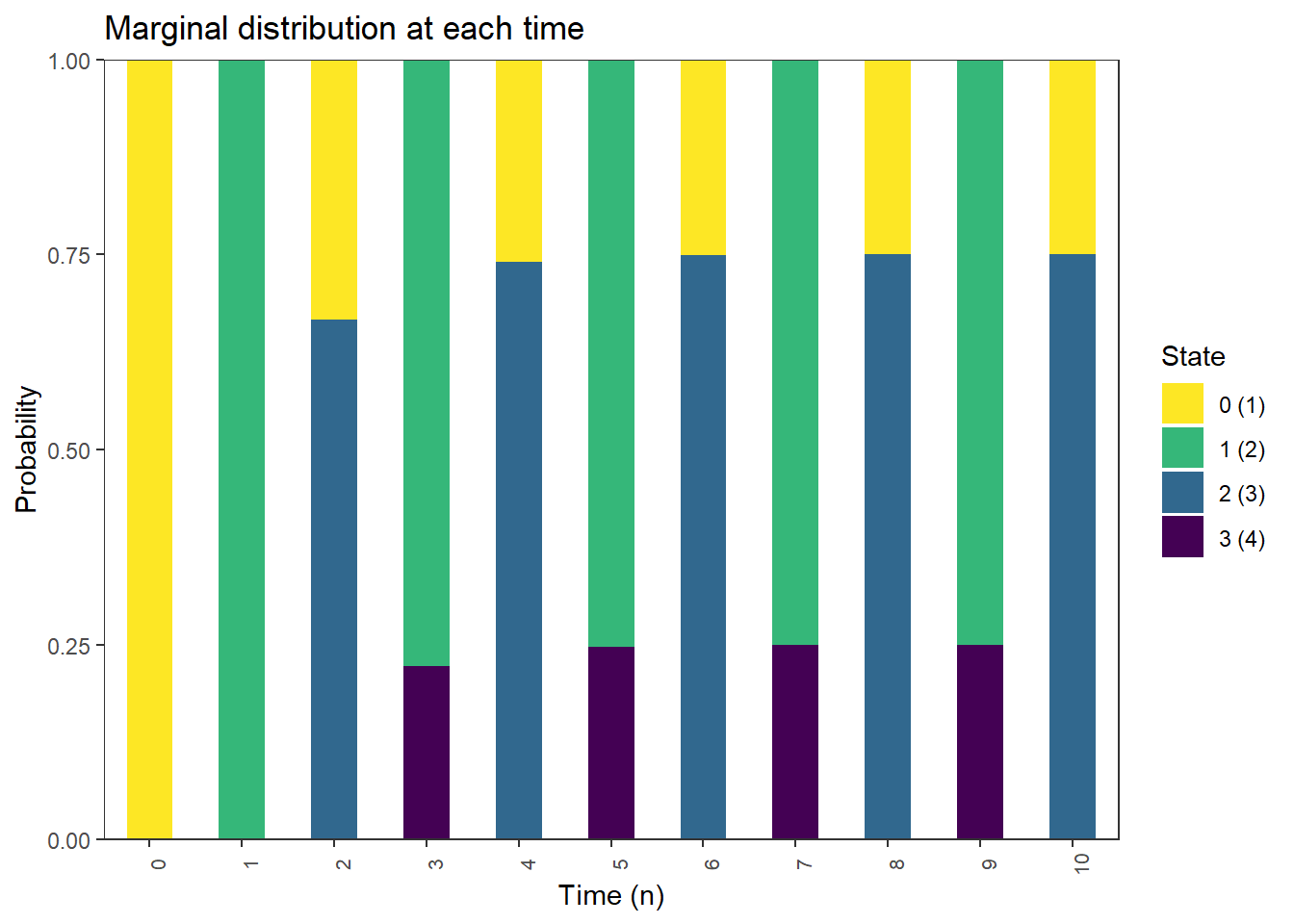
Molecules initially all in B
Marginal distribution of \(X_0\)
pi_0 = c(1, rep(0, M))

pi_0
[1] 1 0 0 0Marginal distribution of \(X_1\)
pi_0 %*% P [,1] [,2] [,3] [,4]
[1,] 0 1 0 0Marginal distribution of \(X_2\)
pi_0 %*% (P %^% 2) [,1] [,2] [,3] [,4]
[1,] 0.3333333 0 0.6666667 0Marginal distribution of \(X_3\)
pi_0 %*% (P %^% 3) [,1] [,2] [,3] [,4]
[1,] 0 0.7777778 0 0.2222222plot_DTMC_marginal_bars(pi_0, P, state_names, last_time = 10)