Introduction to Markov Chain Monte Carlo (MCMC) Methods
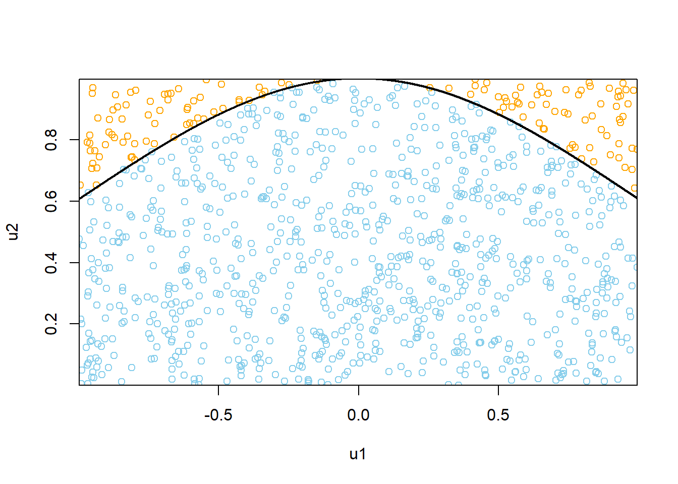
Monte Carlo Integration
The true value of \(\int_{-1}^1 e^{-x^2/2}dx\) is 1.7112488
1000 simulated reps
N =1000# simulate values uniformly in the boxu1 =runif(N, -1, 1)u2 =runif(N, 0, 1)# find the proportion of values that lie under the curve# and multiple by the area of the boxI =2*sum( u2 <exp(-u1 ^2/2)) / NI
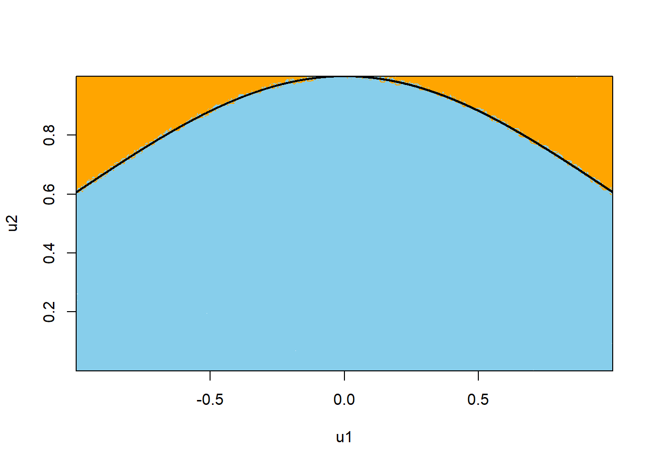
N =100000# simulate values uniformly in the boxu1 =runif(N, -1, 1)u2 =runif(N, 0, 1)# find the proportion of values that lie under the curve# and multiple by the area of the boxI =2*sum( u2 <exp(-u1 ^2/2)) / NI
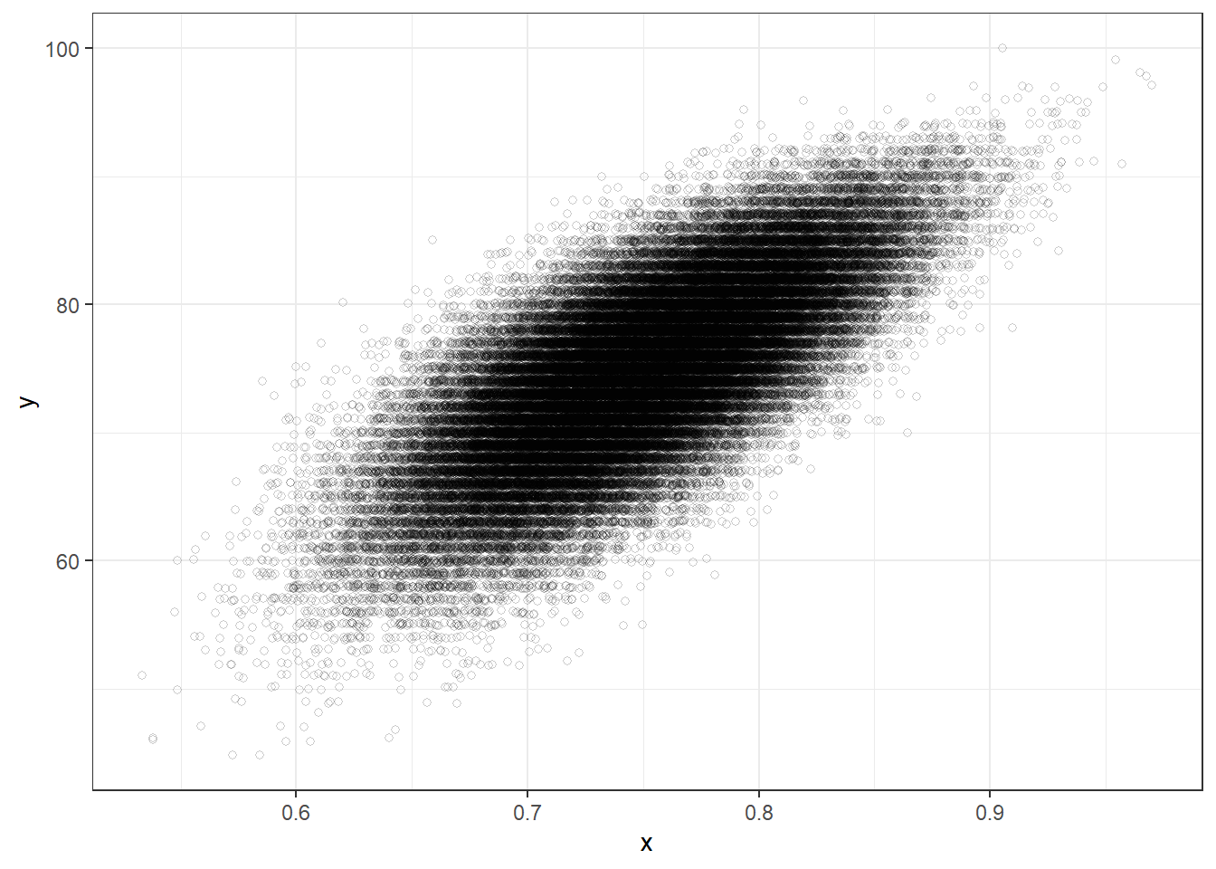
n =100n_rep =100000# Simulate values of X from the marginal distributionx_sim =rnorm(n_rep, 0.75, 0.05)# For each simulated value of x, simulate a value of y from Binomial(n, x)y_sim =rbinom(n_rep, n, x_sim)sim =data.frame(x_sim, y_sim)# Display the (x, y) results of a few repetitionssim |>head(10) |>kbl() |>kable_styling()
# Observed datay_obs =60# Only keep simulated (x, y) pairs with y = 60sim |>filter(y_sim == y_obs) |>head(10) |>kbl() |>kable_styling()
x_sim
y_sim
0.7013796
60
0.7385782
60
0.6319136
60
0.6542770
60
0.7027279
60
0.6477597
60
0.6601650
60
0.6739087
60
0.6698551
60
0.6421359
60
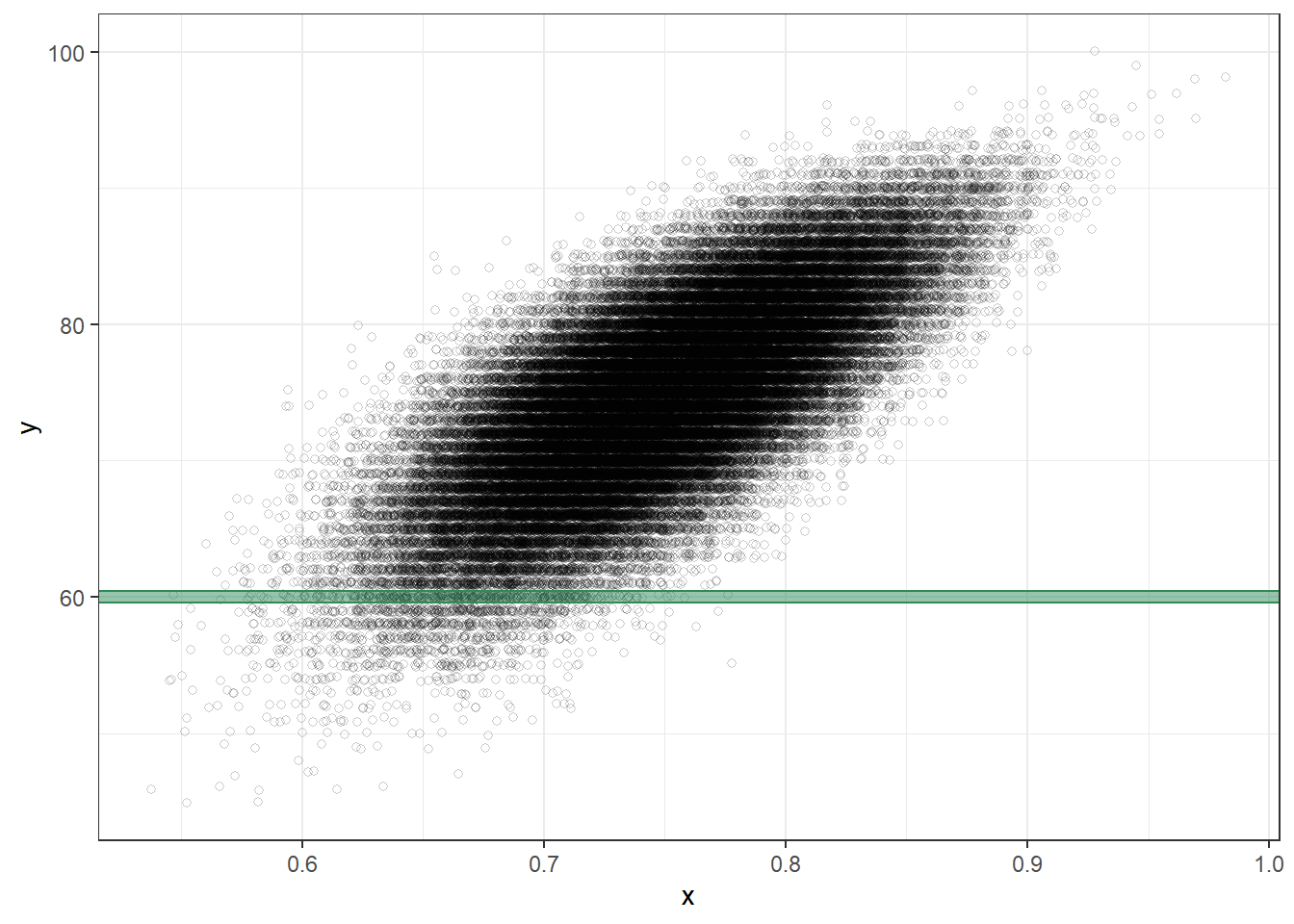
Approximate joint distribution with condition highlighted
# Plot the simulated (x, y) pairs from before, with y = 60 highlightedx_y_plot +annotate("rect", xmin =-Inf, xmax =Inf,ymin = y_obs -0.4, ymax = y_obs +0.4, alpha =0.5,color ="seagreen",fill ="seagreen")
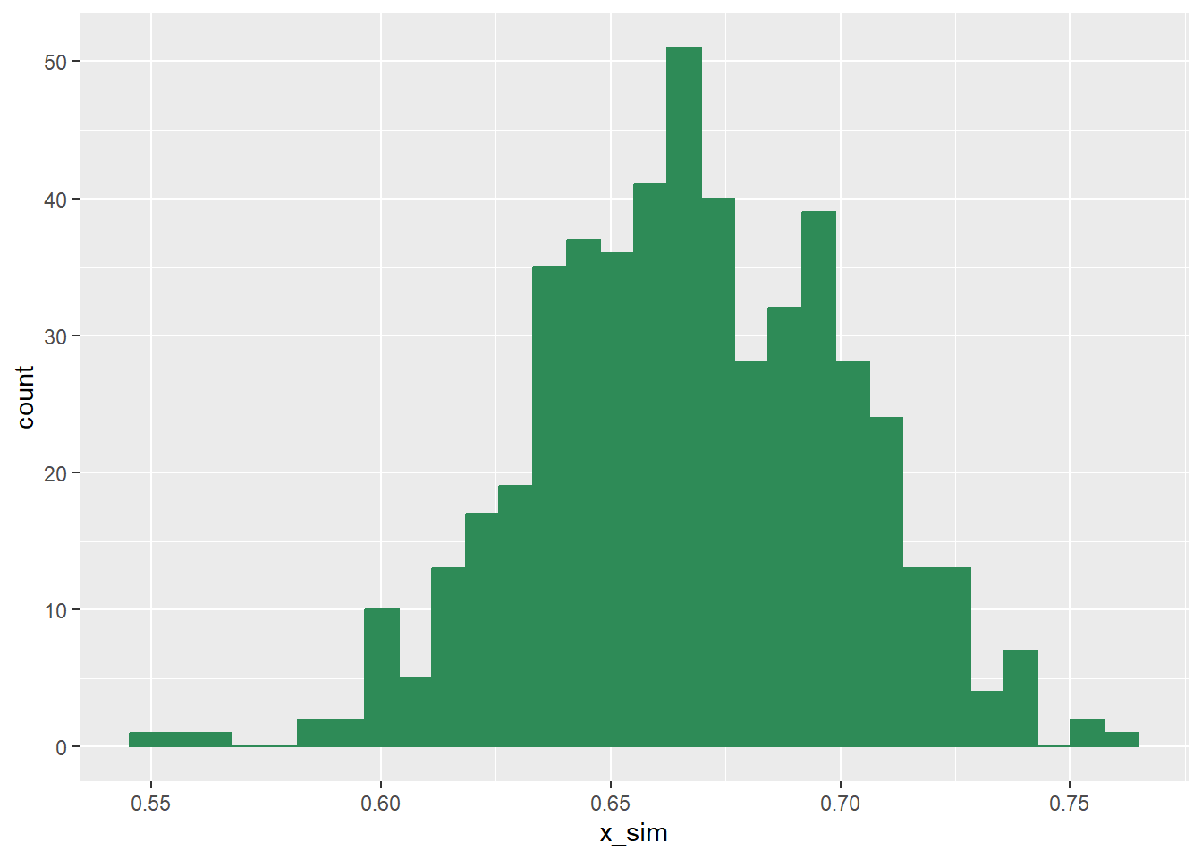
Approximate conditional distribution
# Plot the simulated conditional distribution of X given y = 60sim |>filter(y_sim == y_obs) |>ggplot(aes(x = x_sim)) +geom_histogram(col ="seagreen", fill ="seagreen")
`stat_bin()` using `bins = 30`. Pick better value with `binwidth`.
Started with 100,000 pairs, but conditional distribution is only based on roughly 500.
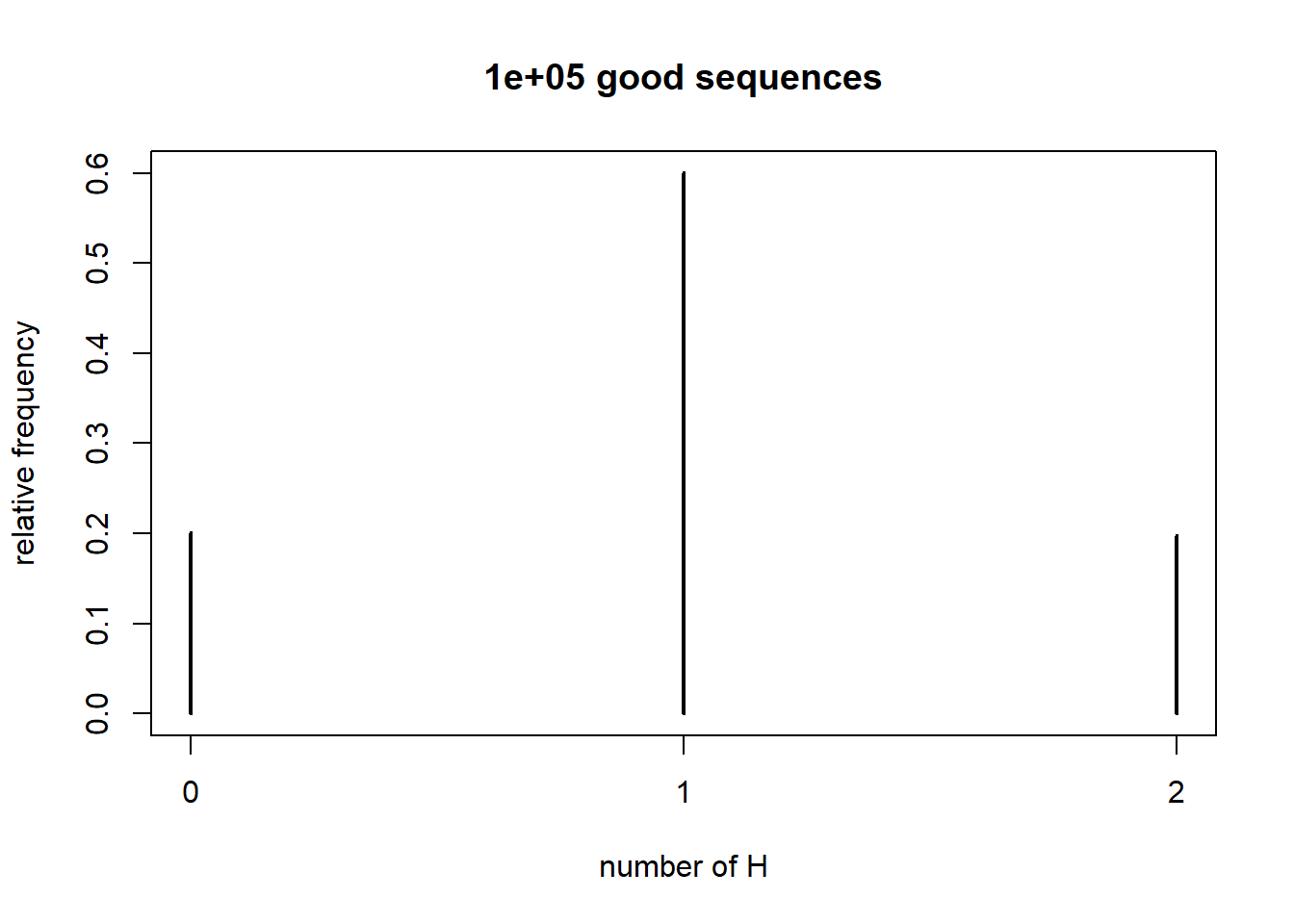
# number of stepsN =100000# number of flipsn =3# initializeXn =matrix(rep(NA, N * n), nrow = N)# start with all tailsXn[1, ] =rep(0, n)for (m in2:N){# current state; all but one flip will stay the same x = Xn[m-1, ]# index of which flip to propose to switch i =sample(1:n, 1) # if proposed switch results in good sequence, accept# otherwise, reject and stay in current state# annoying code for endpointsif (x[i] ==1){ x[i] =0 }else{ #if x[i]==0if((i ==1&& x[i+1] ==0) || (i == n && x[i-1] ==0) || (i>1&& i<n && x[i-1] ==0&& x[i+1] ==0)){ x[i] =1 } else { x[i] =0 } } Xn[m, ] = x}# find number of headsY =rowSums(Xn)plot(table(Y) / N, xlab ="number of H",ylab ="relative frequency",main =paste(N, "good sequences"))
mean(Y)
[1] 0.99665
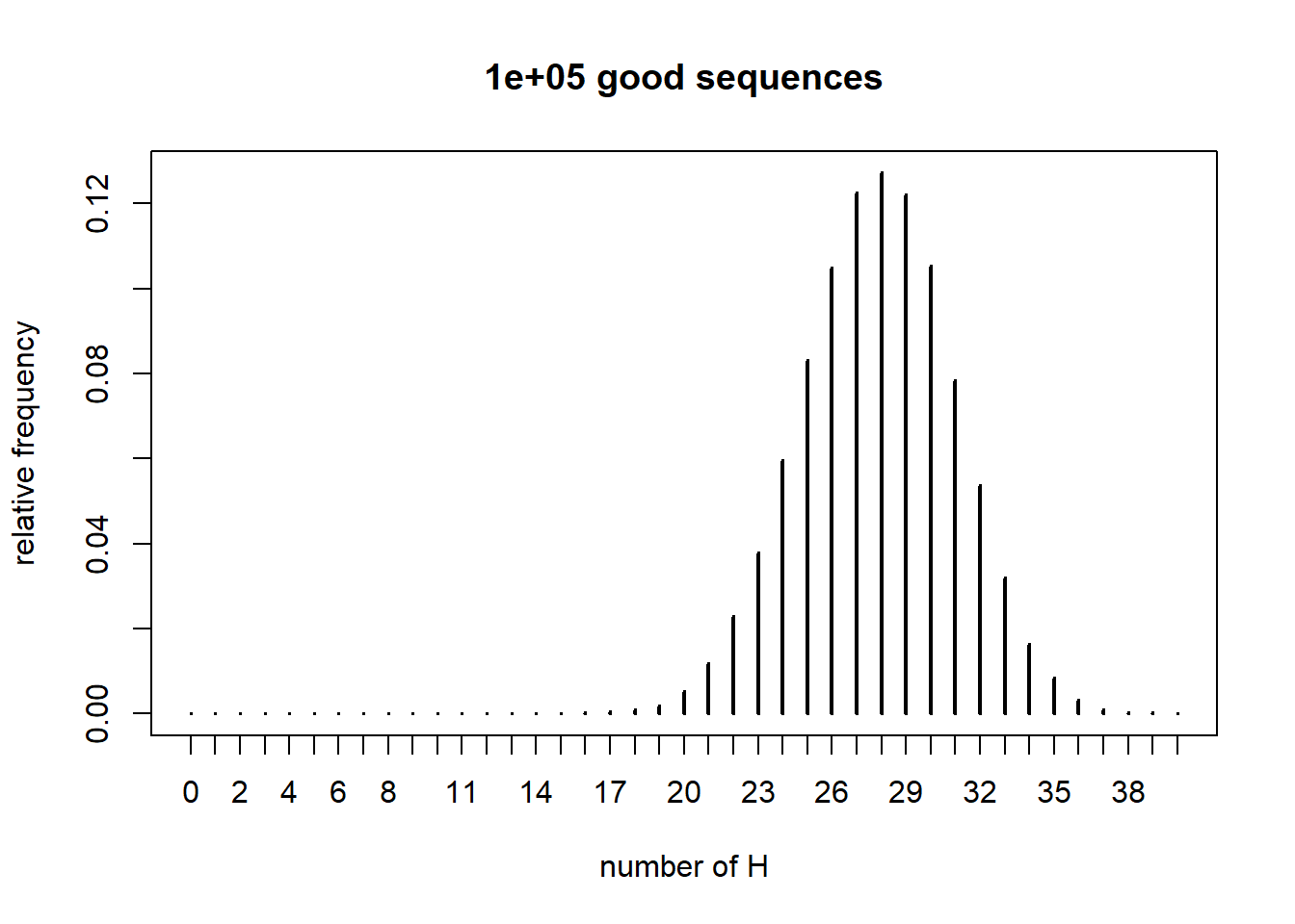
100 flips - same code, just changing 3 to 100
# number of stepsN =100000# number of flipsn =100# initializeXn =matrix(rep(NA, N * n), nrow = N)# start with all tailsXn[1, ] =rep(0, n)for (m in2:N){# current state; all but one flip will stay the same x = Xn[m-1, ]# index of which flip to propose to switch i =sample(1:n, 1) # if proposed switch results in good sequence, accept# otherwise, reject and stay in current state# annoying code for endpointsif (x[i] ==1){ x[i] =0 }else{ #if x[i]==0if((i ==1&& x[i+1] ==0) || (i == n && x[i-1] ==0) || (i>1&& i<n && x[i-1] ==0&& x[i+1] ==0)){ x[i] =1 } else { x[i] =0 } } Xn[m, ] = x}# find number of headsY =rowSums(Xn)plot(table(Y) / N, xlab ="number of H",ylab ="relative frequency",main =paste(N, "good sequences"))