Exponential Distributions

Exponential distributions

from matplotlib import pyplot as plt

from symbulate import *

W = RV(Exponential(rate = 1 / 30))

w = W.sim(10000)

w

Index	Result
0	49.03697641809597
1	9.423805751154866
2	132.84656955378057
3	70.0802876942785
4	42.8600187361989
5	68.94044192928088
6	14.5918468329616
7	9.185332844731454
8	11.33988064850317
...	...
9999	37.85308078050787

plt.figure();

w.plot()

Exponential(rate = 1 / 30).plot()

<symbulate.distributions.Exponential object at 0x000002292F167050>

plt.show();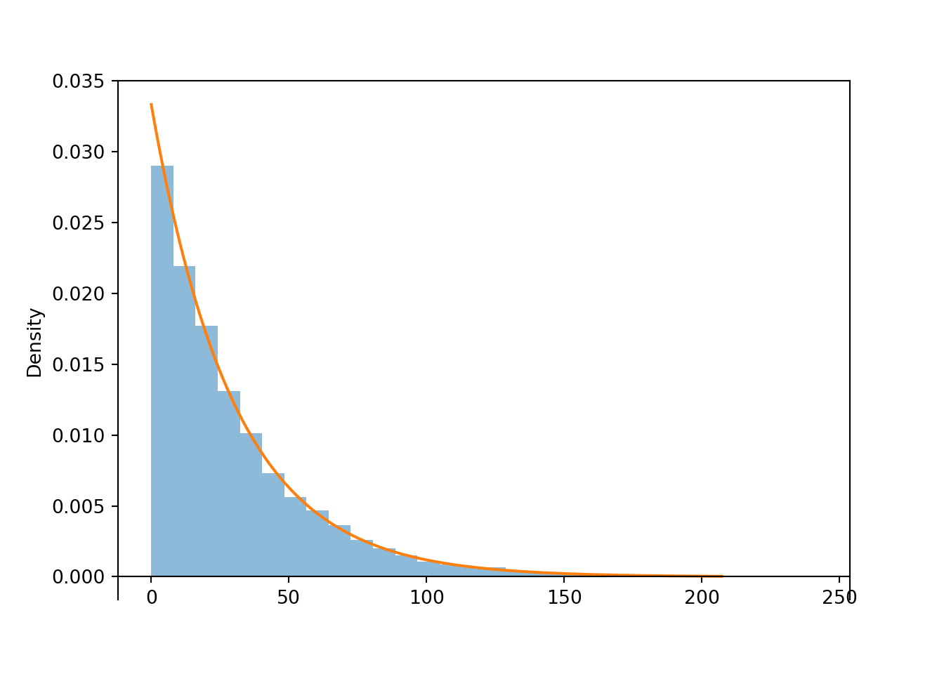

w.count_gt(45) / 10000, 1 - Exponential(rate = 1 / 30).cdf(45)

(0.2228, 0.2231301601484298)

Scaling

U = RV(Exponential(rate = 1))

W = U / (1 / 30)

plt.figure(); 

W.sim(10000).plot()

Exponential(rate = 1 / 30).plot()

<symbulate.distributions.Exponential object at 0x000002292F9232D0>

plt.show();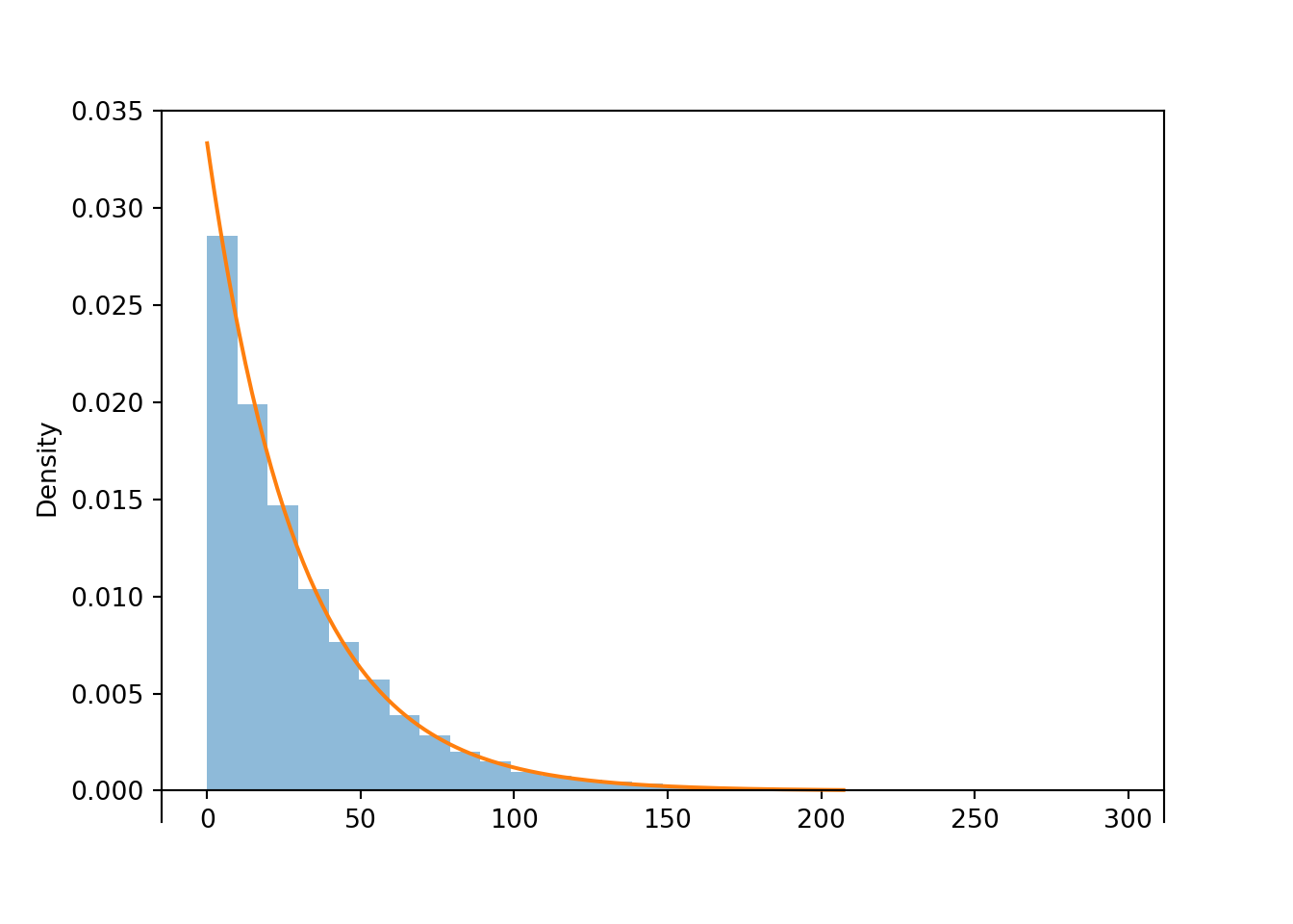

U = RV(Exponential(rate = 1))

V = U / 2

plt.figure(); 

V.sim(10000).plot()

Exponential(rate = 2).plot()

<symbulate.distributions.Exponential object at 0x000002292F92E690>

plt.show();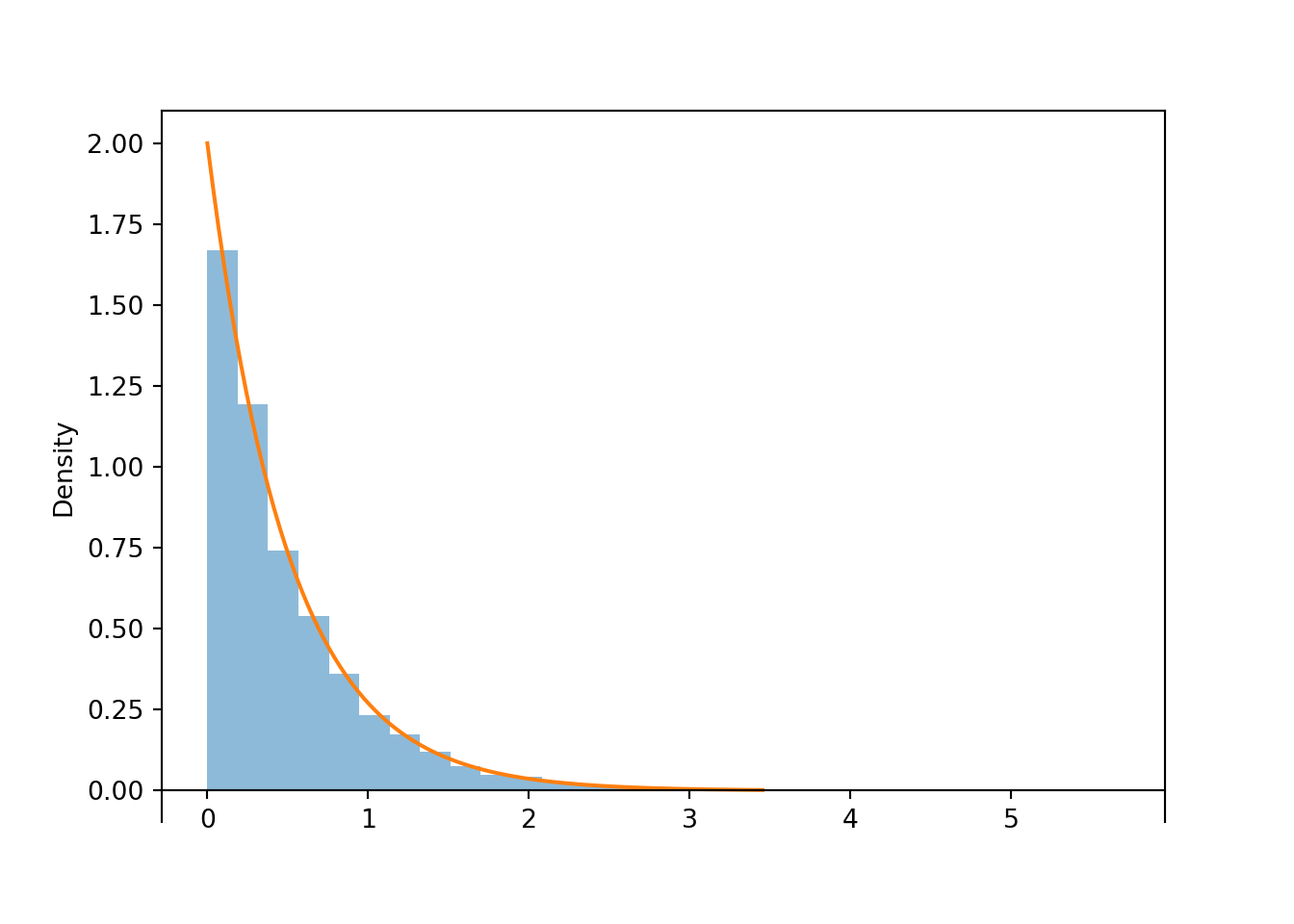

Memoryless property

plt.figure();

W.sim(10000).plot()

(W - 120 | (W > 120) ).sim(10000).plot()

plt.show();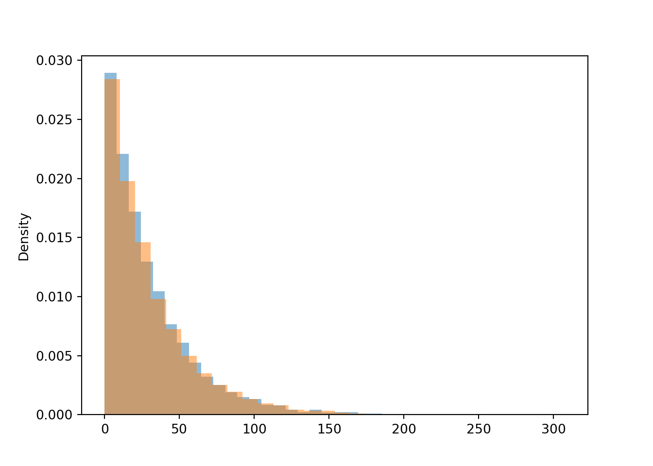

Exponential race

X, Y = RV(Exponential(rate = 1 / 10) * Exponential(rate = 1 / 20))

W = (X & Y).apply(min)

xyw = (X & Y & W).sim(10000)
xyw

Index	Result
0	(1.6897804494190363, 54.251047424807496, 1.6897804494190363)
1	(21.073127016462692, 4.314201032443291, 4.314201032443291)
2	(5.150354478281881, 8.002545837169222, 5.150354478281881)
3	(5.443860882110773, 5.104369643190124, 5.104369643190124)
4	(7.477603528806048, 41.27253893283148, 7.477603528806048)
5	(18.56071637256133, 19.615344156346342, 18.56071637256133)
6	(5.202180555170194, 18.687985339922577, 5.202180555170194)
7	(14.114926015285025, 7.864018408834395, 7.864018408834395)
8	(5.377075413545369, 79.7288284761082, 5.377075413545369)
...	...
9999	(4.389065449318251, 7.465365345227921, 4.389065449318251)

xyw.mean()

(9.935651845714911, 20.161492769314357, 6.595751715218697)

plt.figure();

W.sim(10000).plot()

Exponential(rate = 1 / 10 + 1 / 20).plot()

<symbulate.distributions.Exponential object at 0x000002292FE7D450>

plt.show();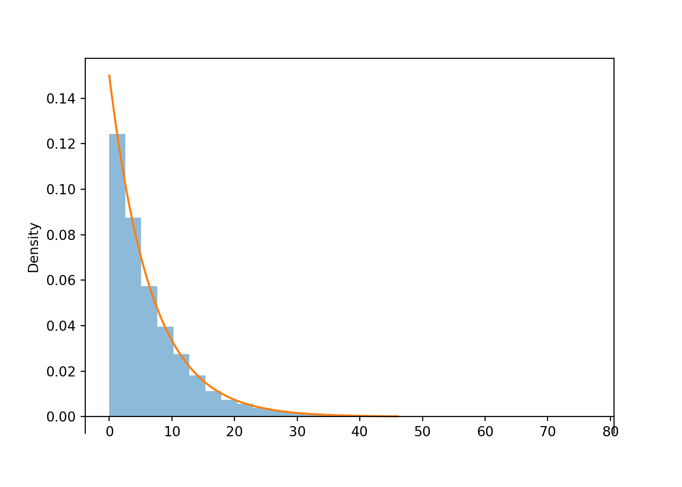

(Y > X).sim(10000).tabulate(normalize = True)

Outcome	Relative Frequency
False	0.329
True	0.671
Total	1.0

plt.figure();

(W | (Y > X) ).sim(10000).plot()

(W | (Y < X) ).sim(10000).plot()

Exponential(rate = 1 / 10 + 1 / 20).plot()

<symbulate.distributions.Exponential object at 0x000002292FB231D0>

plt.show();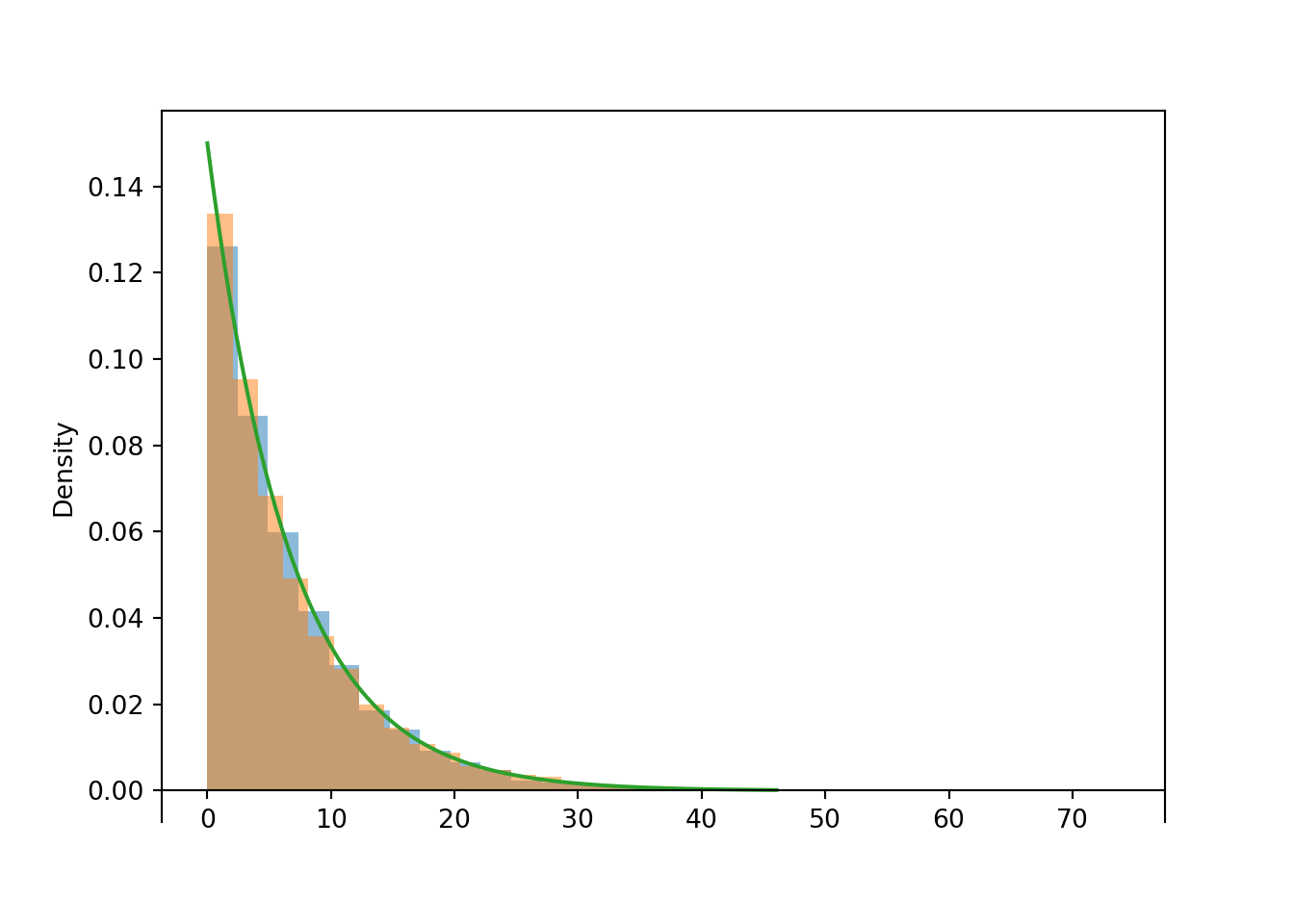

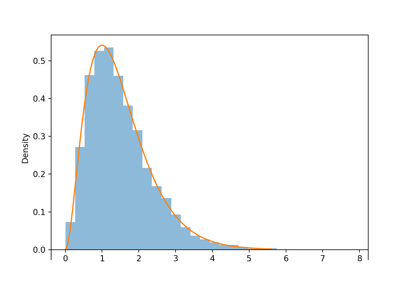
Gamma distributions

W1, W2, W3 = RV(Exponential(rate = 2) ** 3)

T = W1 + W2 + W3

sim = (W1 & W2 & W3 & T).sim(10000)

sim

Index	Result
0	(0.06469452124560411, 1.7855682081667332, 0.5313631202689882, 2.3816258496813254)
1	(0.1584208969802546, 0.4924251031702411, 0.1163766244406055, 0.7672226245911011)
2	(1.0698065892178952, 0.07795530155530278, 0.16496695664767727, 1.3127288474208751)
3	(0.21436431905901593, 0.5583898831088366, 0.016993425807202714, 0.7897476279750554)
4	(0.0005713850629777853, 0.3881865649738012, 1.510141515540344, 1.898899465577123)
5	(0.012704265881709228, 0.4672657986103173, 0.19088675080722023, 0.6708568152992468)
6	(0.045426184155089054, 0.7530210654992747, 0.3150977064163982, 1.113544956070762)
7	(0.4596560710480708, 0.28077703838656387, 0.23965647395637424, 0.9800895833910089)
8	(0.9467156208910521, 1.0575805333836266, 0.24898627141401772, 2.2532824256886963)
...	...
9999	(0.8860052047301088, 0.060700238141574506, 0.537647553037698, 1.4843529959093813)

sim.mean()

(0.5007131157254108, 0.5000359531826972, 0.513057655279491, 1.5138067241875979)

sim.var()

(0.24657422498246614, 0.24389642533279743, 0.261121071967302, 0.7693369341430786)

sim.sd()

(0.49656240794331796, 0.4938587098885646, 0.5110000704180989, 0.8771185405309129)

plt.figure();

T.sim(10000).plot()

Gamma(shape = 3, rate = 2).plot()

<symbulate.distributions.Gamma object at 0x000002292FAC1F50>

plt.show();