Metropolis-Hastings Algorithm

Island hopping

# states
n_states = 30
i = 1:n_states

# target distribution - proportional to
pi_i = i ^ 2 * exp(-0.5 * i) # notice: not probabilities

n_steps = 10000
i_sim = rep(NA, n_steps)
i_sim[1] = 3 # initialize

for (n in 2:n_steps){
  current = i_sim[n - 1]
  
  # propose next state
  proposed = sample(c(current + 1, current - 1), size = 1, prob = c(0.5, 0.5))
  
  # compute acceptance probability
  if (!(proposed %in% i)){ # to correct for proposing moves outside of boundaries
proposed = current
  }
  a = min(1, pi_i[proposed] / pi_i[current])
  
  # simulate the next state
  i_sim[n] = sample(c(proposed, current), size = 1, prob = c(a, 1 - a))
}

First few steps

# display the first few steps
data.frame(step = 1:n_steps, i_sim) |> head(10) |> kbl() |> kable_styling() 

step	i_sim
1	3
2	2
3	2
4	3
5	2
6	2
7	3
8	3
9	4
10	5

First 100 steps

# trace plot
plot(1:100, i_sim[1:100], type = "o",
     ylim = range(i), xlab = "Day", ylab = "Island")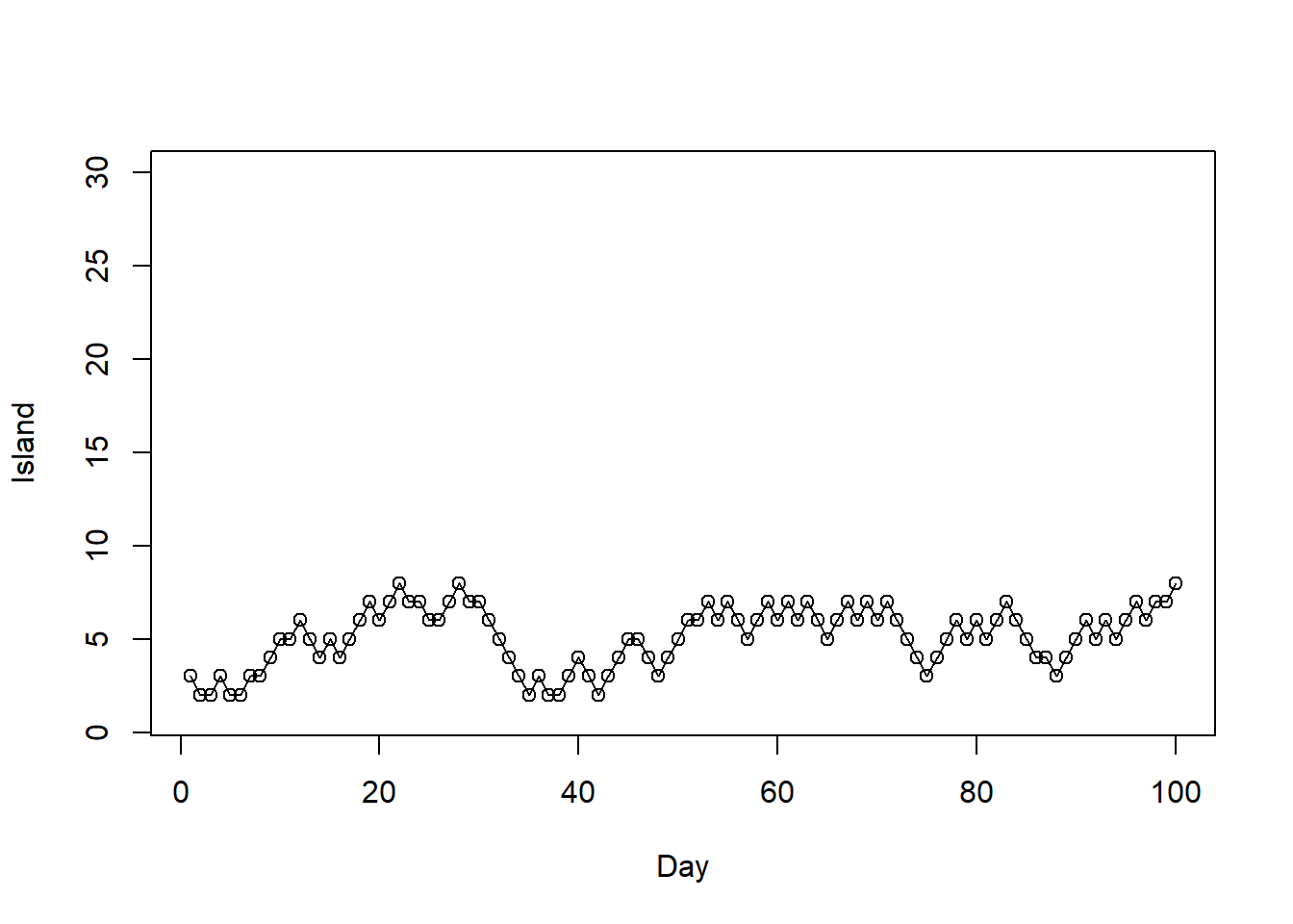

Relative frequencies of first 100 steps

# simulated relative frequencies
plot(table(i_sim[1:100]) / 100,
     xlab = "Island", ylab = "Proportion of days")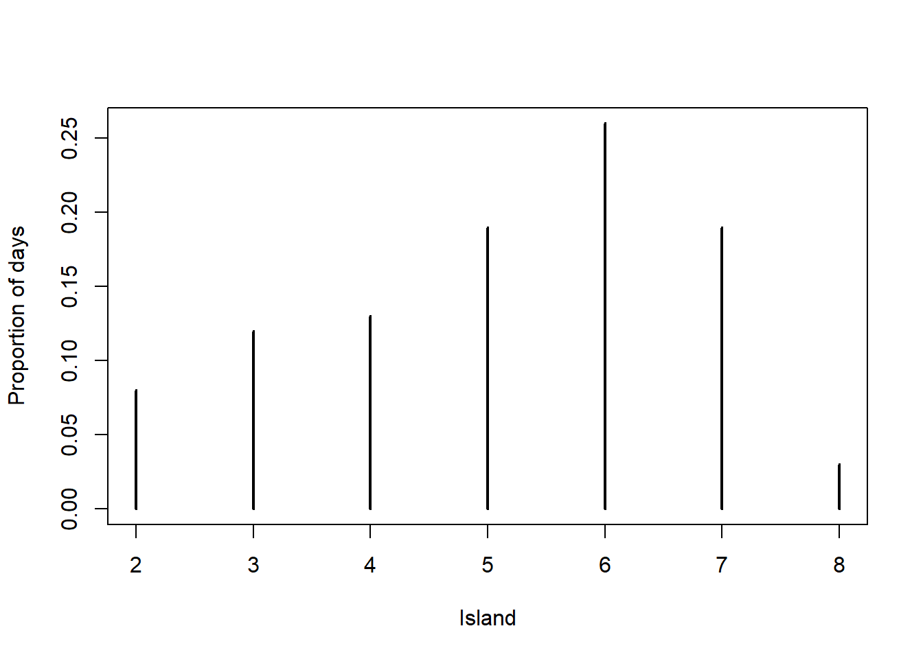

First 10000 steps

# trace plot
plot(1:n_steps, i_sim, type = "l",
     ylim = range(i), xlab = "Day", ylab = "Island")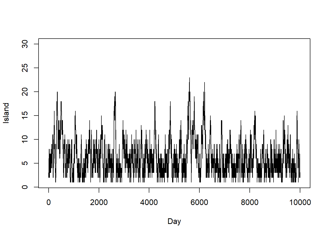

Relative frequencies of first 10000 steps

# simulated relative frequencies
plot(table(i_sim) / n_steps,
     xlab = "Island", ylab = "Proportion of days")

# target distribution
points(i, pi_i / sum(pi_i), type = "o",
       col = "seagreen")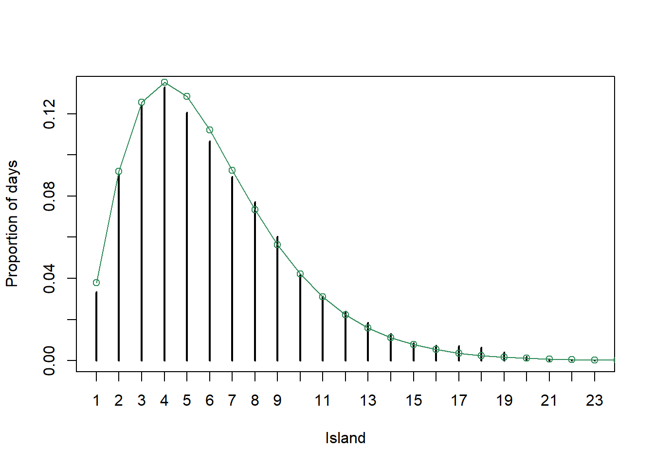

Explicit M-H transition matrix

P = rbind(
  c(0.5, 0.5, 0),
  c(0.25, 0.25, 0.5),
  c(0, 1 / 3, 2 / 3)
)

compute_stationary_distribution(P)

          [,1]      [,2] [,3]
[1,] 0.1666667 0.3333333  0.5

Zipf

# parameters of Zipf
alpha = 1
M = 10
states = 1:M

# proposal chain is random walk (with reflection at boundaries)
pup = 0.5
Q = matrix(rep(0, M * M), nrow = M)

Q[1, 1] = 1 - pup
Q[1, 2] = pup
Q[M, M] = pup
Q[M, M - 1] = 1 - pup
for (i in 2:(M - 1)){
  Q[i, i - 1] = 1 - pup
  Q[i, i + 1] = pup
}

# Metropolis-Hastings chain
N = 10000
Xn = rep(NA, N)
Xn[1] = 1

for (n in 2:N){
  # current state
  i = Xn[n - 1]
  
  # proposed state
  j = sample(states, 1 , prob = Q[i, ])
  
  # acceptance probability
  aij = min(1, (1 / j) ^ alpha / (1 / i) ^ alpha)
  
  # next state - accept j or stay at i
  Xn[n] = sample(c(i, j), 1, prob = c(1 - aij, aij)) 
}

# trace plot
plot(1:N, Xn, type = "l",
     ylim = range(states), xlab = "n", ylab = "X_n")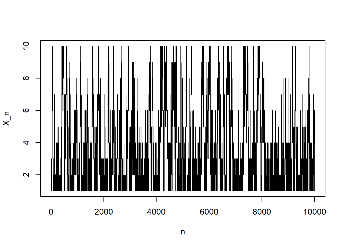

# simulated relative frequencies
plot(table(Xn) / N,
     xlab = "x", ylab = "Relative frequency")

# target Zipf distribution
pi_x = (1 / states) ^ alpha
pi_x = pi_x / sum(pi_x)

points(states, pi_x, type = "o",
       col = "seagreen")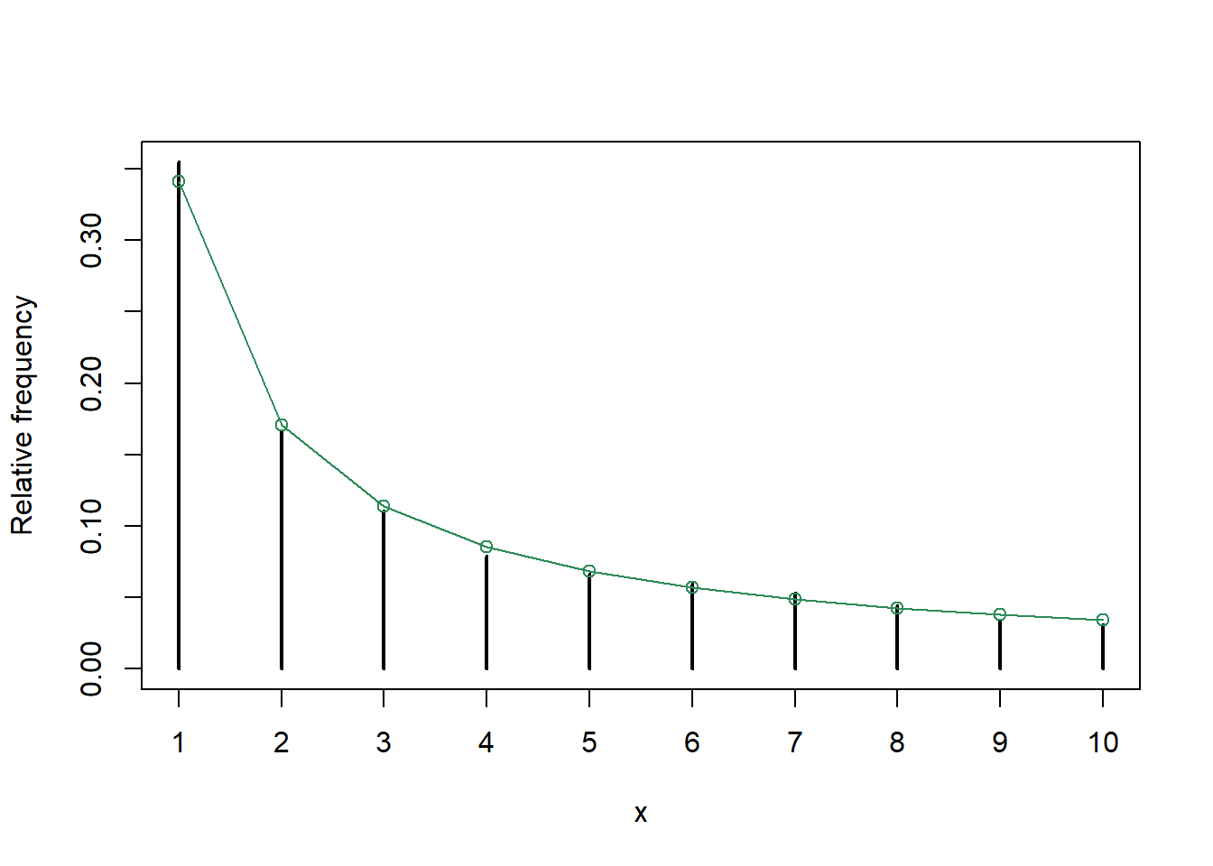

Gamma

Normal proposals

pi_x = function(u) {
  if (u > 0) {
    u ^ (7.2 - 1) * exp(-3 * u)
  } else {
    0
  }
}

sigma = 0.5

N = 10000


x_n = rep(NA, N)
x_n[1] = 4

for (i in 2:N){
  current = x_n[i-1]
  proposed = rnorm(1, current, sigma)
  a = min(1, pi_x(proposed) / pi_x(current))
  x_n[i] = sample(c(current, proposed), 1, prob = c(1 - a, a)) 
}

plot(1:N, x_n , type="l", xlab = "n", ylab = "X_n")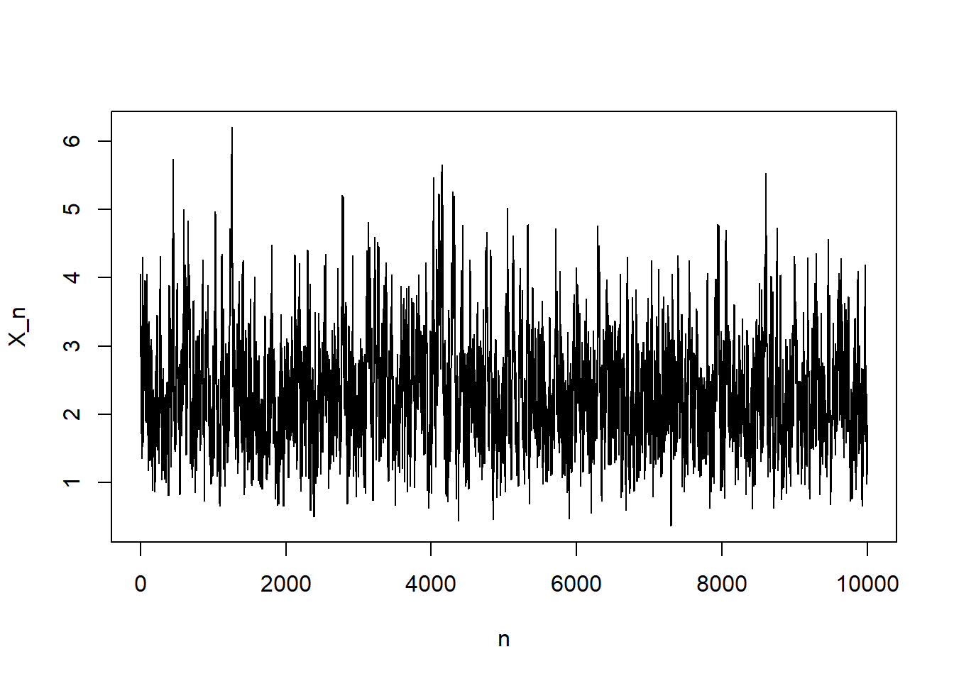

hist(x_n, freq = FALSE)
curve(dgamma(x, shape = 7.2, rate = 3), add = TRUE, col = "seagreen")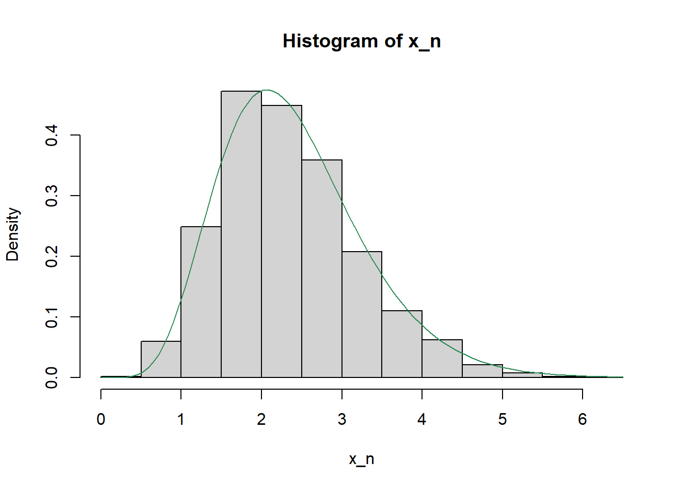

Moving Uniform proposals

delta = 0.5

N = 10000

x_n = rep(NA, N)
x_n[1] = 4

for (i in 2:N){
  current = x_n[i-1]
  proposed = runif(1, current - delta, current + delta)
  a = min(1, pi_x(proposed) / pi_x(current))
  x_n[i] = sample(c(current, proposed), 1, prob = c(1 - a, a)) 
}

plot(1:N, x_n , type="l", xlab = "n", ylab = "X_n")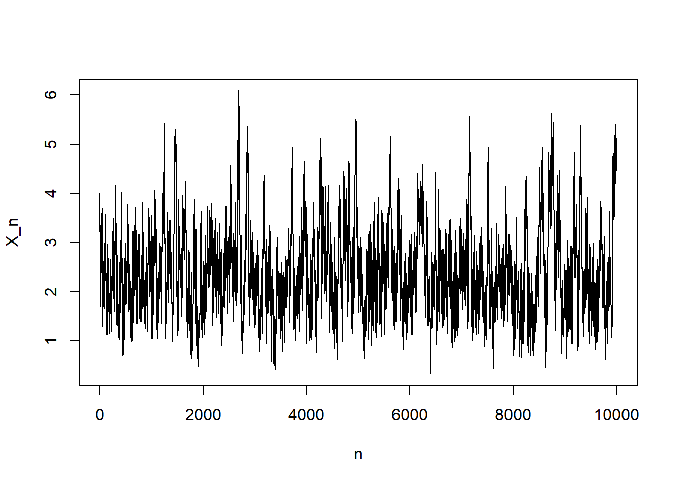

hist(x_n, freq = FALSE)
curve(dgamma(x, shape = 7.2, rate = 3), add = TRUE, col = "seagreen")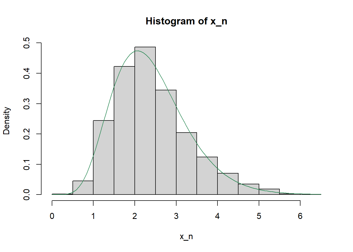

Multivariable

Normal proposals

pi_xy = function(x, y) {
  if ((x > 0) & (y > 0)) {
    exp(-(x + y + x * y))
  } else {
    0
  }
}

sigma = 0.5

N = 10000


x_n = rep(NA, N)
y_n = rep(NA, N)
x_n[1] = 1
y_n[1] = 1

for (i in 2:N){
  current_x = x_n[i-1]
  current_y = y_n[i-1]
  
  proposed_x = rnorm(1, current_x, sigma)
  proposed_y = rnorm(1, current_y, sigma)
  
  a = min(1, pi_xy(proposed_x, proposed_y) / pi_xy(current_x, current_y))
  action = sample(c("reject", "accept"), 1, prob = c(1 - a, a))
  
  if (action == "accept"){
    x_n[i] = proposed_x
    y_n[i] = proposed_y
  } else {
    x_n[i] = current_x
    y_n[i] = current_y
  }
}

plot(x_n, y_n)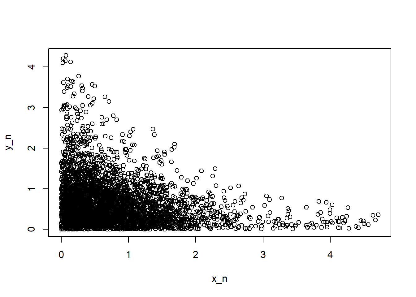

# Trace plot of first 100 steps
xy = data.frame(x_n, y_n)

ggplot(xy[1:100, ] |>
         mutate(label = 1:100),
       aes(x_n, y_n)) +
  geom_path() +
  geom_point(size = 2) +
  geom_text(aes(label = label, x = x_n + 0.1, y = y_n + 0.01)) +
  labs(title = "Trace plot of first 100 steps")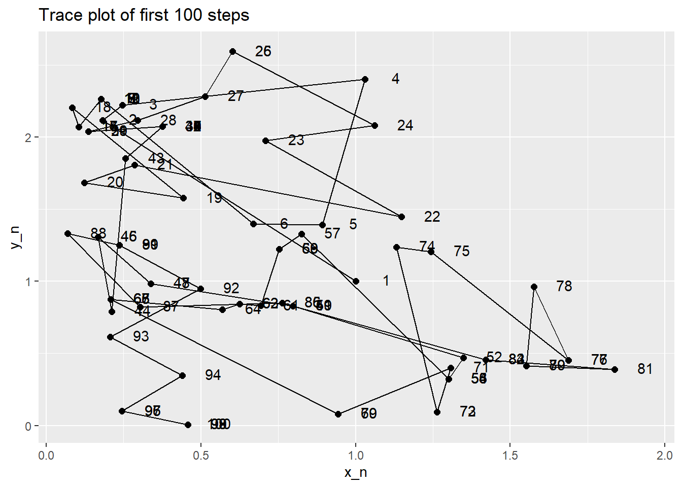

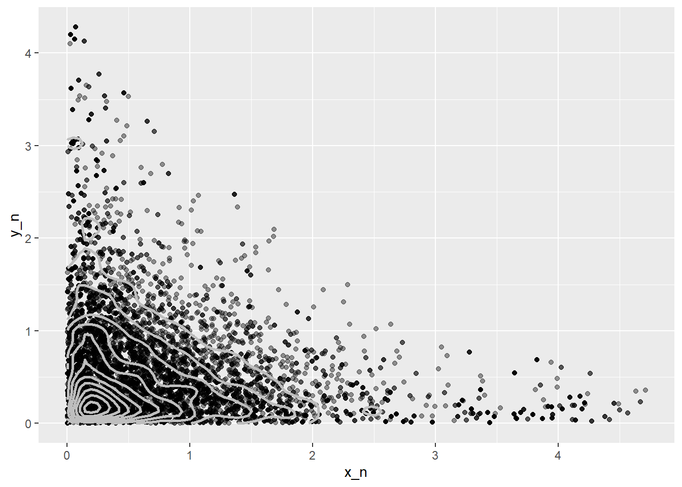
ggplot(xy, aes(x_n, y_n)) +
  geom_point(alpha = 0.4) +
  stat_density_2d(color = "grey", size = 1)

Warning: Using `size` aesthetic for lines was deprecated in ggplot2 3.4.0.
ℹ Please use `linewidth` instead.