Discrete Time Markov Chains: Long Run Behavior

Recurrent and transient states example

P = rbind(
  c(0, 1, 0, 0, 0, 0),
  c(0, 0, 1, 0, 0, 0),
  c(0.7, 0, 0, 0.3, 0, 0),
  c(0, 0, 0, 0, 1, 0),
  c(0, 0, 0, 0.3, 0, 0.7),
  c(0, 0, 0, 0.8, 0, 0.2)
)

plot_state_diagram(P)

Joining with `by = join_by(prob)`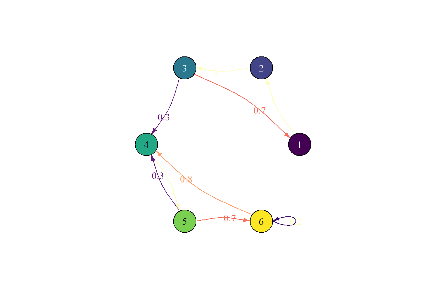

plot_sample_path_proportions(c(1, 0, 0, 0, 0, 0), P, last_time = 1000)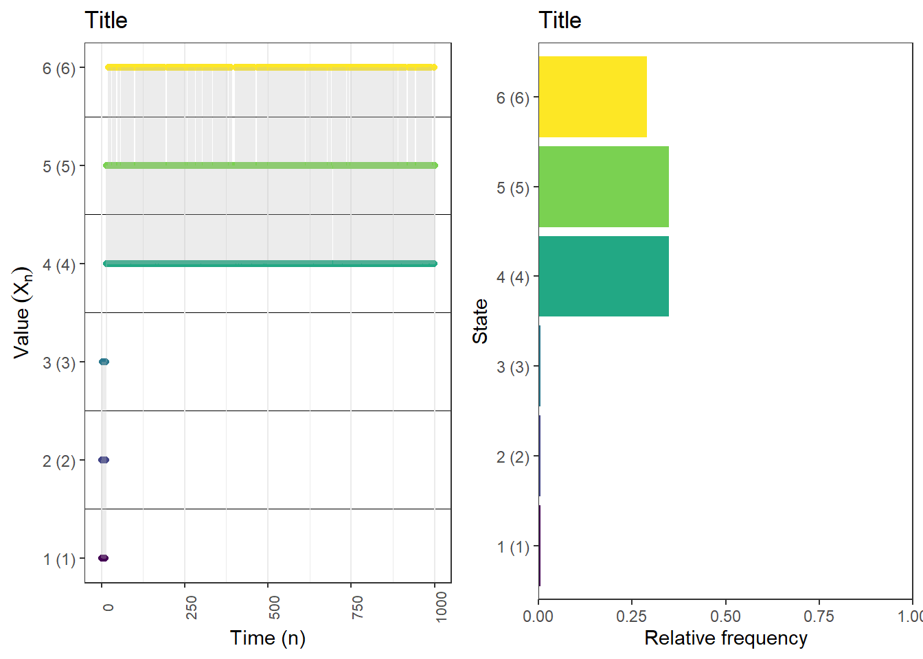

Compute stationary distribution for the recurrent states

compute_stationary_distribution(P[4:6, 4:6])

          [,1]      [,2]      [,3]
[1,] 0.3478261 0.3478261 0.3043478

Markov’s letters

state_names = c("vowel", "consonant")

P = rbind(
  c(0.128, 0.872),
  c(0.663, 0.337)
)

pi_0 = c(1, 0)

plot_sample_path_proportions(pi_0, P, state_names, last_time = 1000)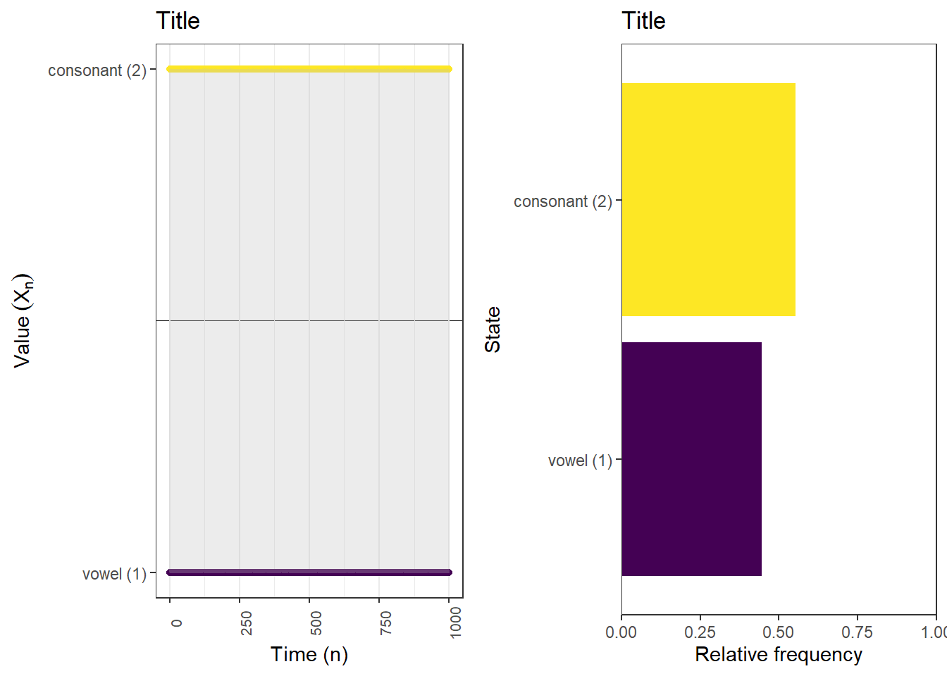

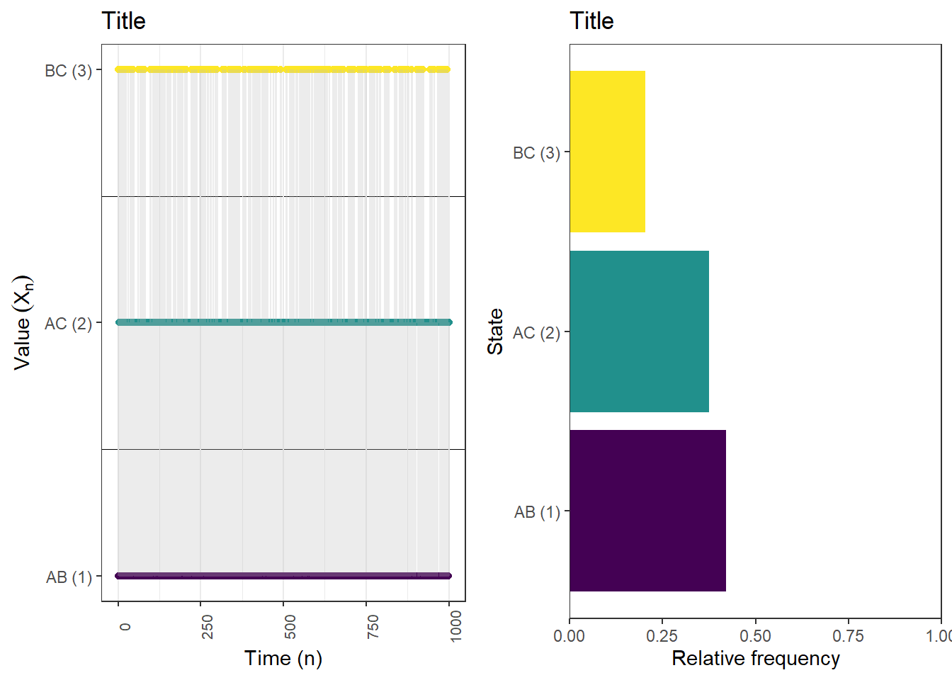
Ping pong

state_names = c("AB", "AC", "BC")

P = rbind(c(0, .7, .3),
          c(.8, 0, .2),
          c(.6, .4, 0)
)

pi_0 = c(1, 0, 0)

plot_sample_path_proportions(pi_0, P, state_names, last_time = 1000)