state_names = c("vowel", "consonant")

P = rbind(
  c(0.128, 0.872),
  c(0.663, 0.337)
)

pi_0 = c(0.432, 0.568)Steady State Distributions
Markov’s letters
1-step transition matrix
plot_transition_matrix(P, state_names)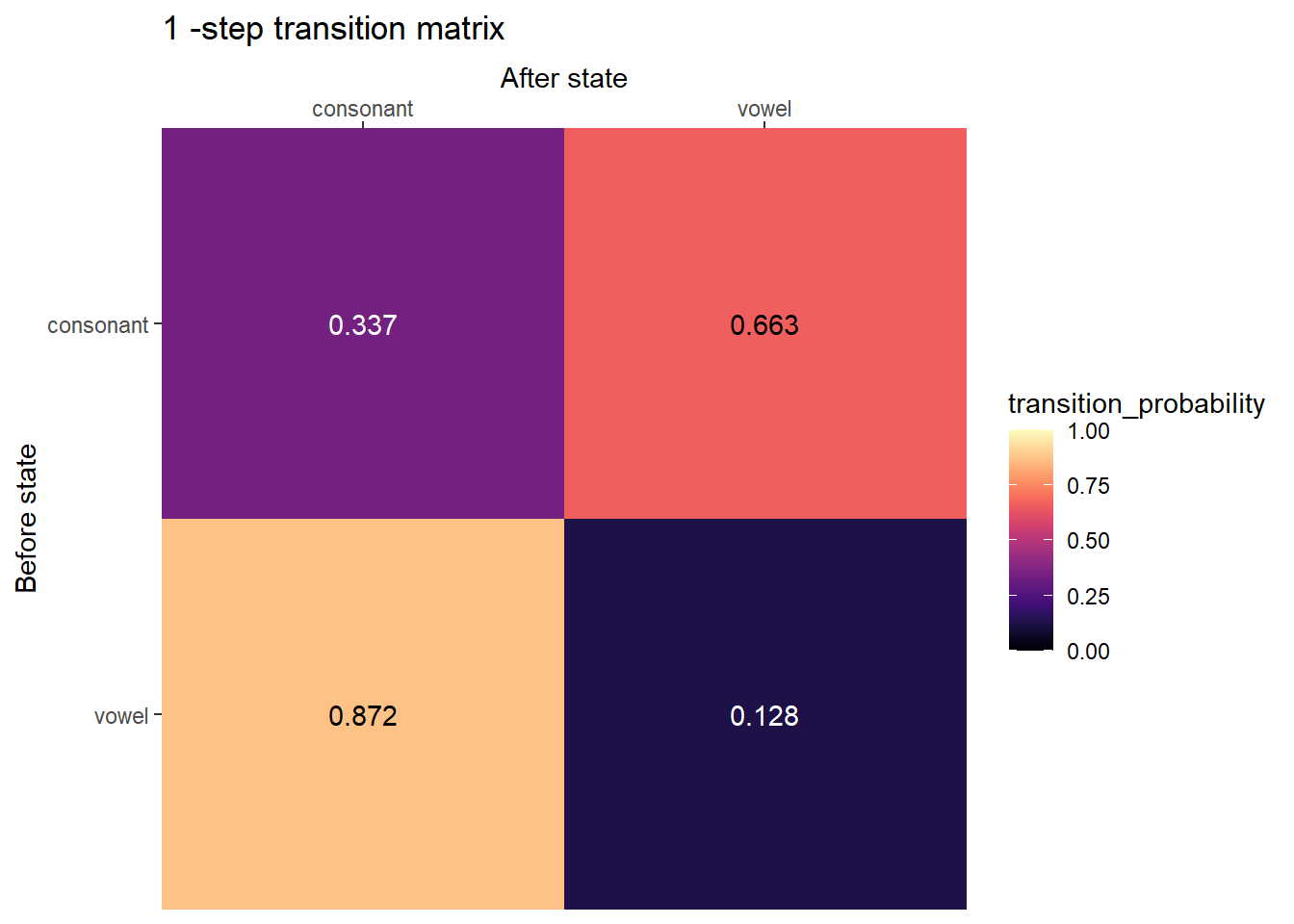
2-step transition matrix
plot_transition_matrix(P, state_names, n_step = 2)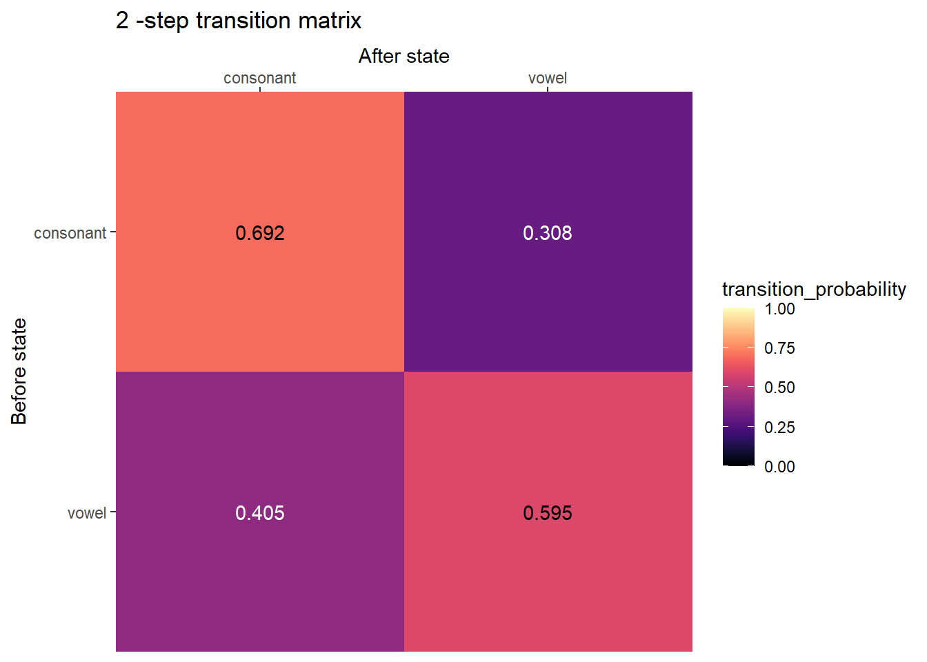
3-step transition matrix
plot_transition_matrix(P, state_names, n_step = 3)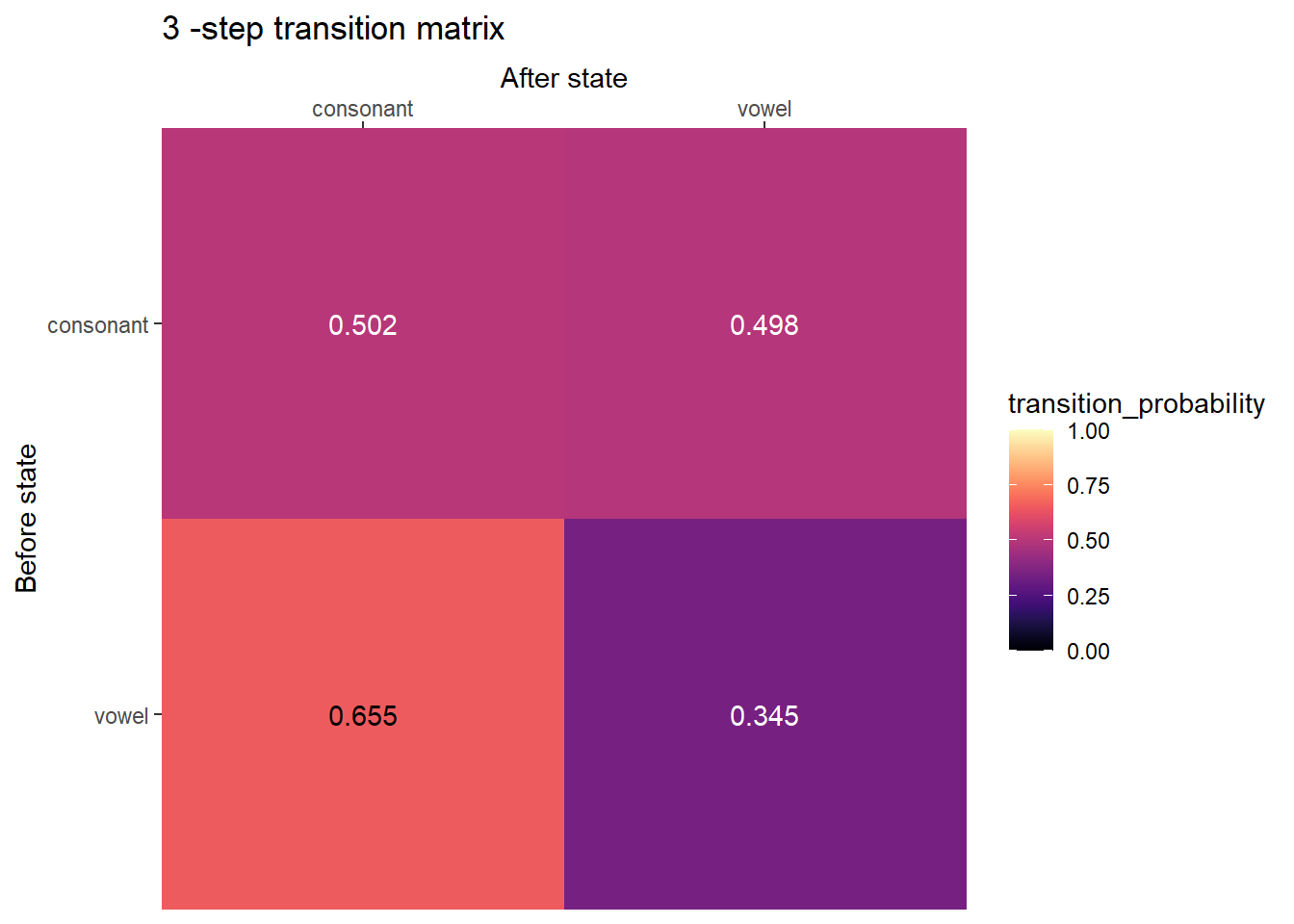
5-step transition matrix
plot_transition_matrix(P, state_names, n_step = 5)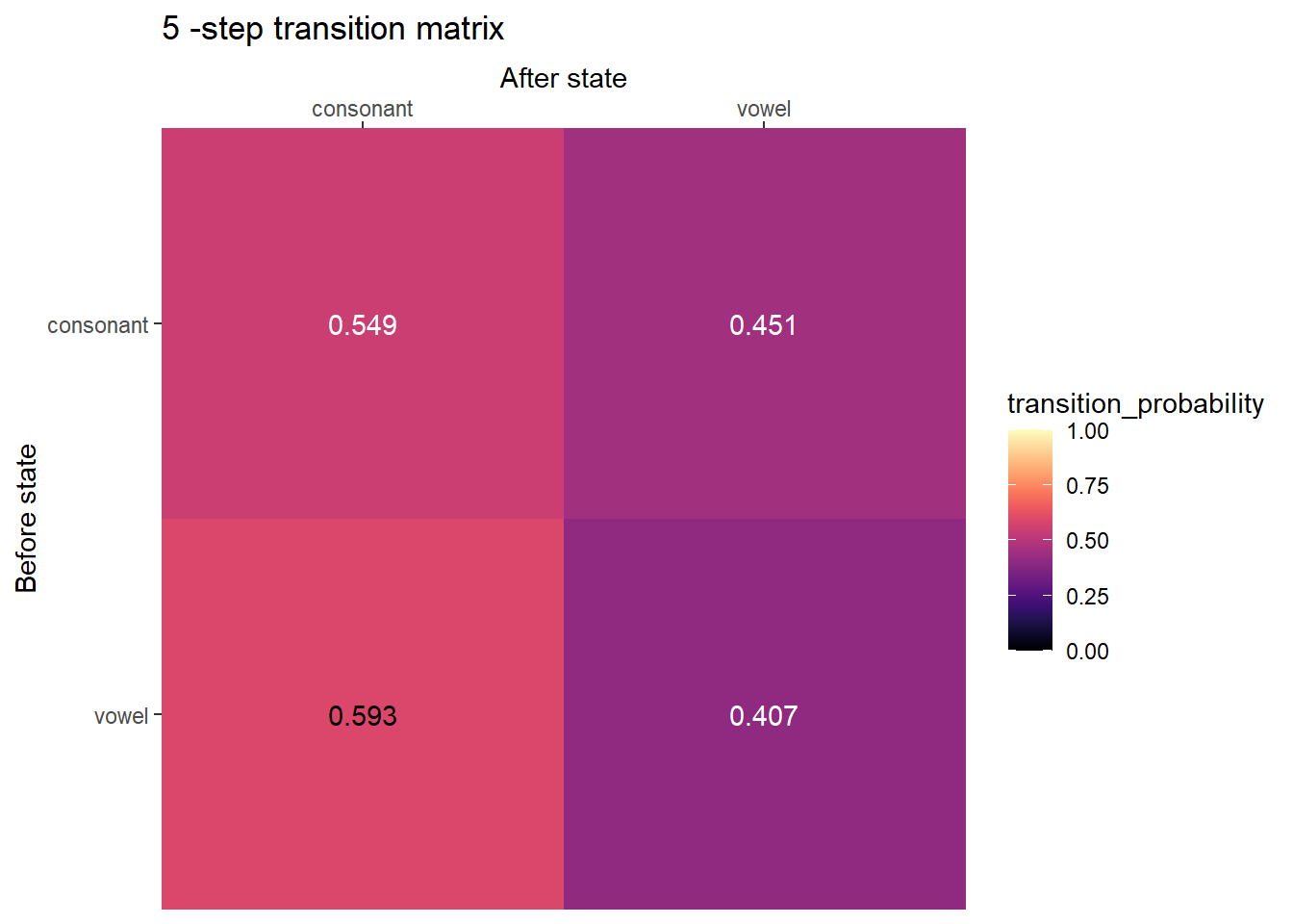
10-step transition matrix
plot_transition_matrix(P, state_names, n_step = 10)
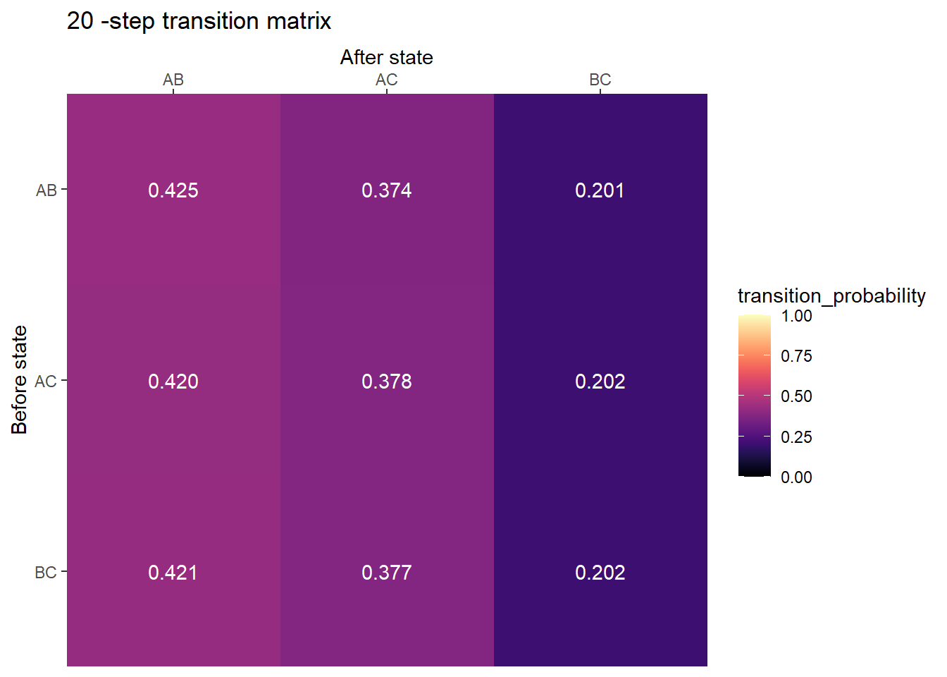
20-step transition matrix
plot_transition_matrix(P, state_names, n_step = 20)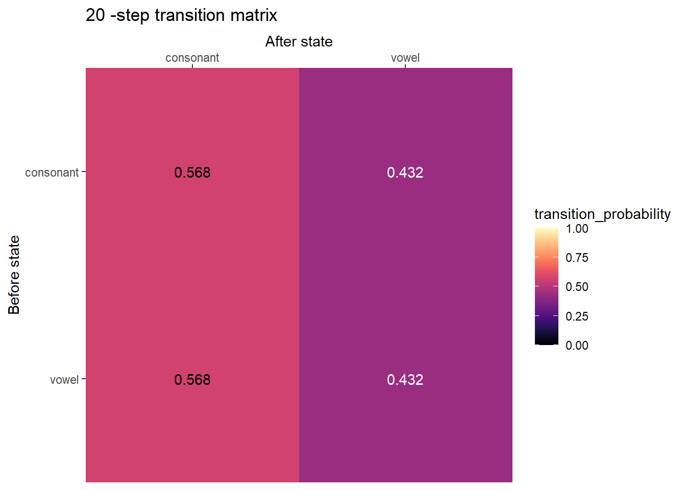
Ehrenfest urn chain
M = 3

state_names = 0:M

P = rbind(c(0, 1, 0, 0),
         c(1/3, 0, 2/3, 0),
         c(0, 2/3, 0, 1/3),
         c(0, 0, 1, 0)
)
100-step transition matrix
plot_transition_matrix(P, state_names, n_step = 100)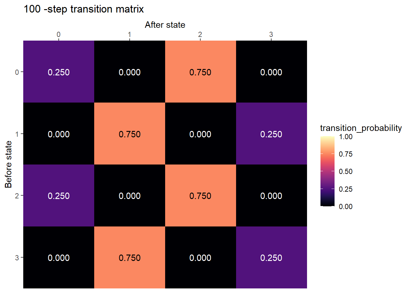
101-step transition matrix
plot_transition_matrix(P, state_names, n_step = 101)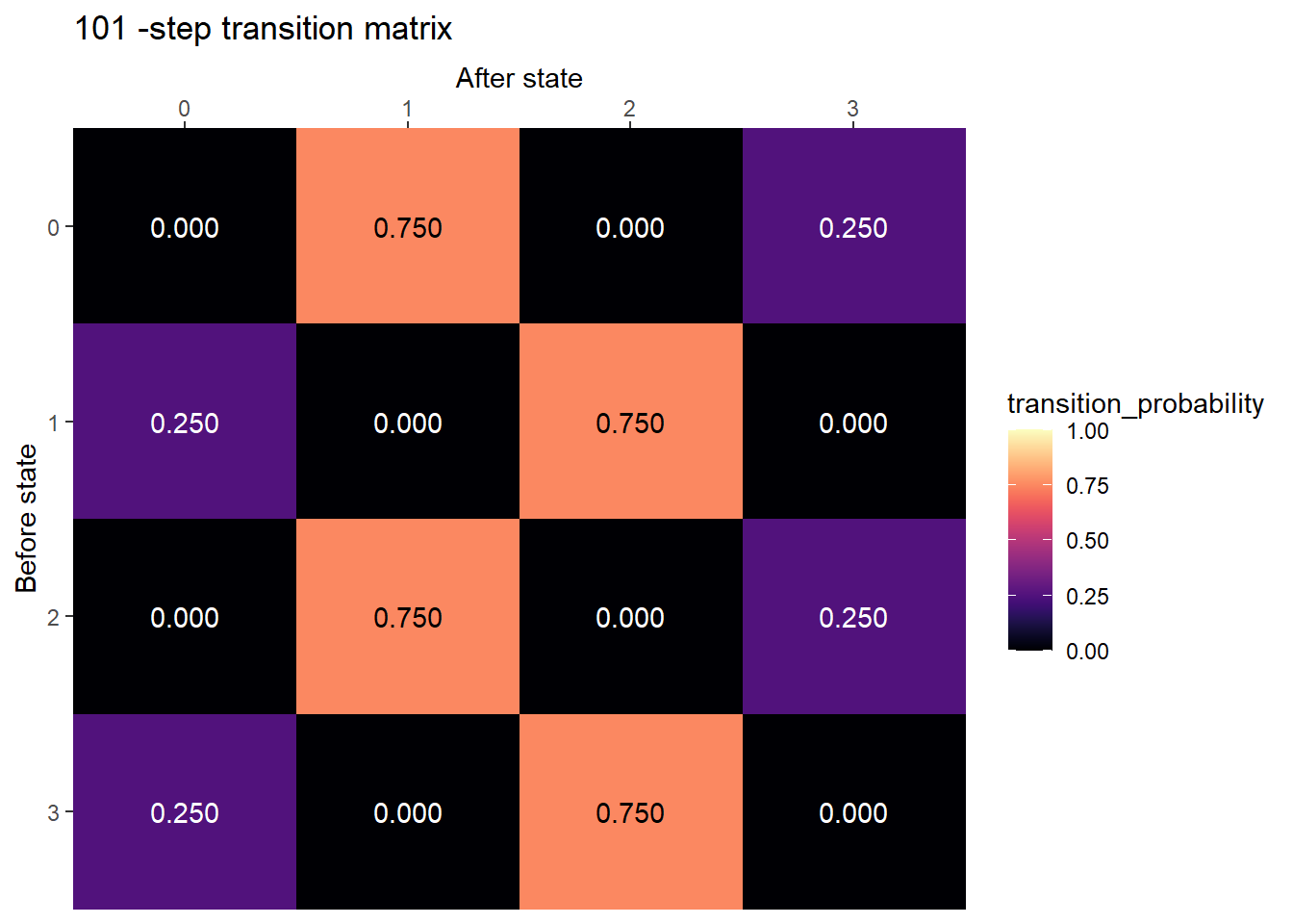
Stationary distribution
pi_s = compute_stationary_distribution(P)

# display in table
data.frame(state_names, t(pi_s)) |>
  kbl(col.names = c("state", "stationary probability")) |>
kable_styling()| state | stationary probability |
|---|---|
| 0 | 0.125 |
| 1 | 0.375 |
| 2 | 0.375 |
| 3 | 0.125 |
Ping pong
state_names = c("AB", "AC", "BC")

P = rbind(c(0, .7, .3),
          c(.8, 0, .2),
          c(.6, .4, 0)
)
Stationry distribution
pi_s = compute_stationary_distribution(P)

# display in table
data.frame(state_names, t(pi_s)) |>
  kbl(col.names = c("state", "stationary probability"), digits = 4) |>
kable_styling()| state | stationary probability |
|---|---|
| AB | 0.4220 |
| AC | 0.3761 |
| BC | 0.2018 |
transition matrix
plot_transition_matrix(P, state_names, n_step = 1)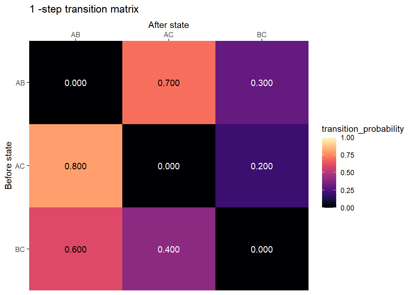
2-step transition matrix
plot_transition_matrix(P, state_names, n_step = 2)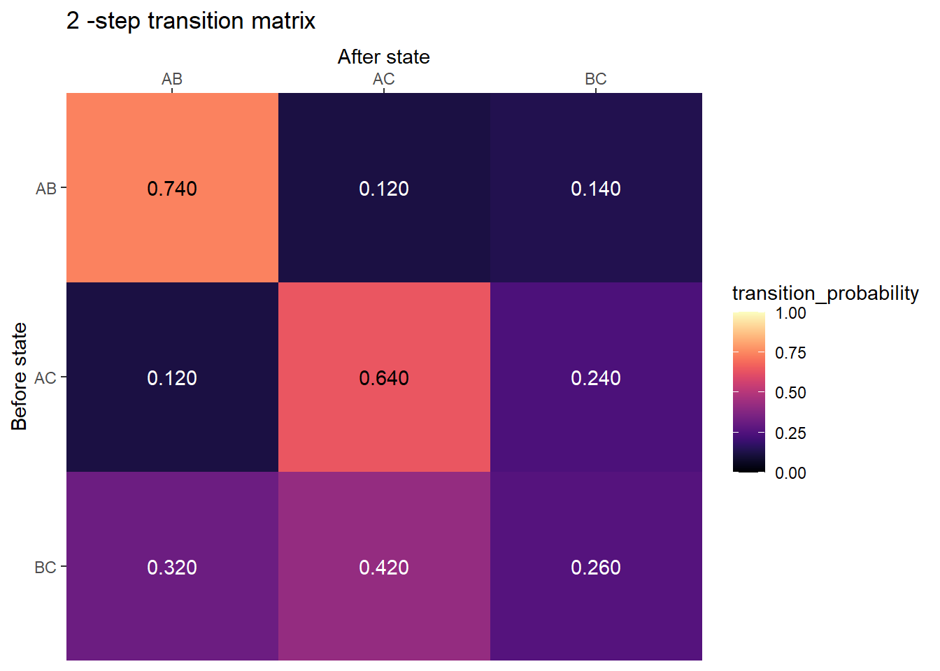
10-step transition matrix
plot_transition_matrix(P, state_names, n_step = 10)
20-step transition matrix
plot_transition_matrix(P, state_names, n_step = 20)