Stationary Distributions

Function to compute stationary distribution for finite state, irreducible transition matrix

compute_stationary_distribution <- function(P){

  s = nrow(P)

  rep(1, s) %*% solve(diag(s) - P + matrix(rep(1, s * s), ncol = s))

}

Markov’s letters

state_names = c("vowel", "consonant")

P = rbind(
  c(0.128, 0.872),
  c(0.663, 0.337)
)

pi_0 = c(0.432, 0.568)

Marginal distributions if initial distribution is stationary distribution

plot_DTMC_marginal_bars(pi_0, P, state_names, last_time = 20)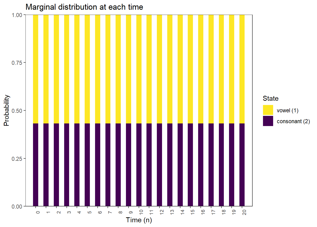

Ehrenfest urn chain

M = 3

state_names = 0:M

P = rbind(c(0, 1, 0, 0),
         c(1/3, 0, 2/3, 0),
         c(0, 2/3, 0, 1/3),
         c(0, 0, 1, 0)
)

Stationary distribution

pi_s = compute_stationary_distribution(P)

# display in table
data.frame(state_names, t(pi_s)) |>
  kbl(col.names = c("state", "stationary probability")) |>
  kable_styling()

state	stationary probability
0	0.125
1	0.375
2	0.375
3	0.125

Marginal distributions if initial distribution is stationary distribution

plot_DTMC_marginal_bars(pi_s, P, state_names, last_time = 20)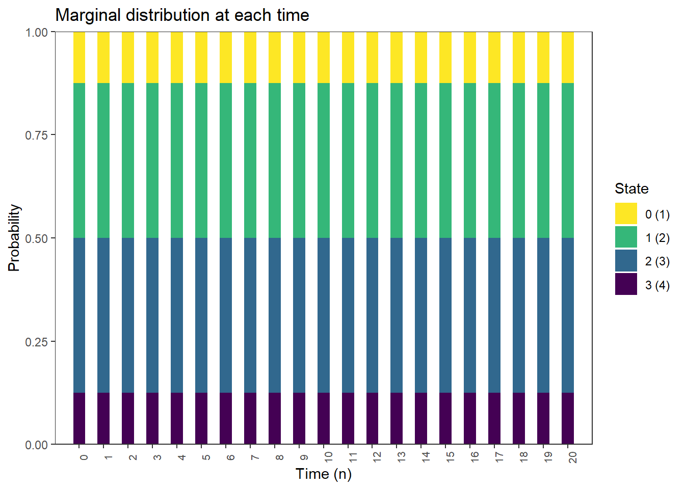

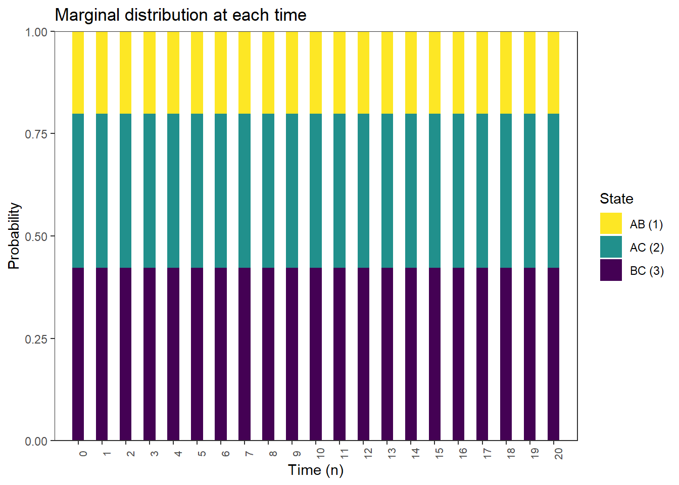
Ping pong

state_names = c("AB", "AC", "BC")

P = rbind(c(0, .7, .3),
          c(.8, 0, .2),
          c(.6, .4, 0)
)

Stationry distribution

pi_s = compute_stationary_distribution(P)

# display in table
data.frame(state_names, t(pi_s)) |>
  kbl(col.names = c("state", "stationary probability"), digits = 4) |>
  kable_styling()

state	stationary probability
AB	0.4220
AC	0.3761
BC	0.2018

Marginal distributions if initial distribution is stationary distribution

plot_DTMC_marginal_bars(pi_s, P, state_names, last_time = 20)