Birth and Death Chains

M/M/1 Queue simulation of long run distribution

lambda = 0.2

mu = 0.5

n_jumps = 10000

X_t = rep(NA, n_jumps + 1)
W_n = rep(NA, n_jumps + 1)
T_n = rep(NA, n_jumps + 1)

X_t[1] = 0
T_n[1] = 0

for (n in 2:(n_jumps + 1)){
  if (X_t[n - 1] == 0){
    W_n[n - 1] = rexp(1) / lambda
    T_n[n] = T_n[n - 1] + W_n[n - 1]
    X_t[n] = X_t[n - 1] + 1
  } else {
    W_n[n - 1] = rexp(1) / (lambda + mu)
    T_n[n] = T_n[n - 1] + W_n[n - 1]
    X_t[n] = X_t[n - 1] + sample(c(-1, 1), 1, prob = c(mu, lambda))
  }
}

plot(T_n, X_t,
     type = "s",
     xlab = "t", ylab = "X(t)",
     main = "Sample path of M/M/1 queue")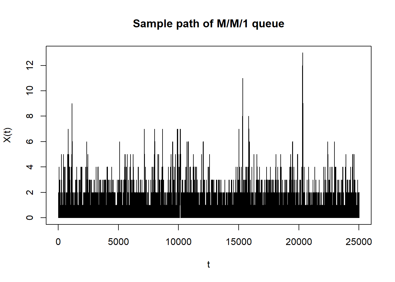

long_run_distribution = data.frame(T_n, X_t, W_n) |>
  slice_head(n = n_jumps) |>
  mutate(total_time = sum(W_n)) |>
  group_by(X_t) |>
  summarize(total_time_in_state = sum(W_n),
            total_time = max(total_time),
            fraction_time_in_state = total_time_in_state / total_time)

long_run_distribution |>
  select(X_t, fraction_time_in_state) |>
  kbl(digits = 3) |> kable_styling()

X_t	fraction_time_in_state
0	0.598
1	0.240
2	0.094
3	0.038
4	0.017
5	0.006
6	0.004
7	0.001
8	0.001
9	0.001
10	0.000
11	0.000
12	0.000
13	0.000

long_run_distribution |>
  ggplot(aes(x = X_t,
             y = fraction_time_in_state)) +
  geom_point() +
  geom_line() +
  labs(x = "State (number in system)",
       y = "Long run fraction of time in state")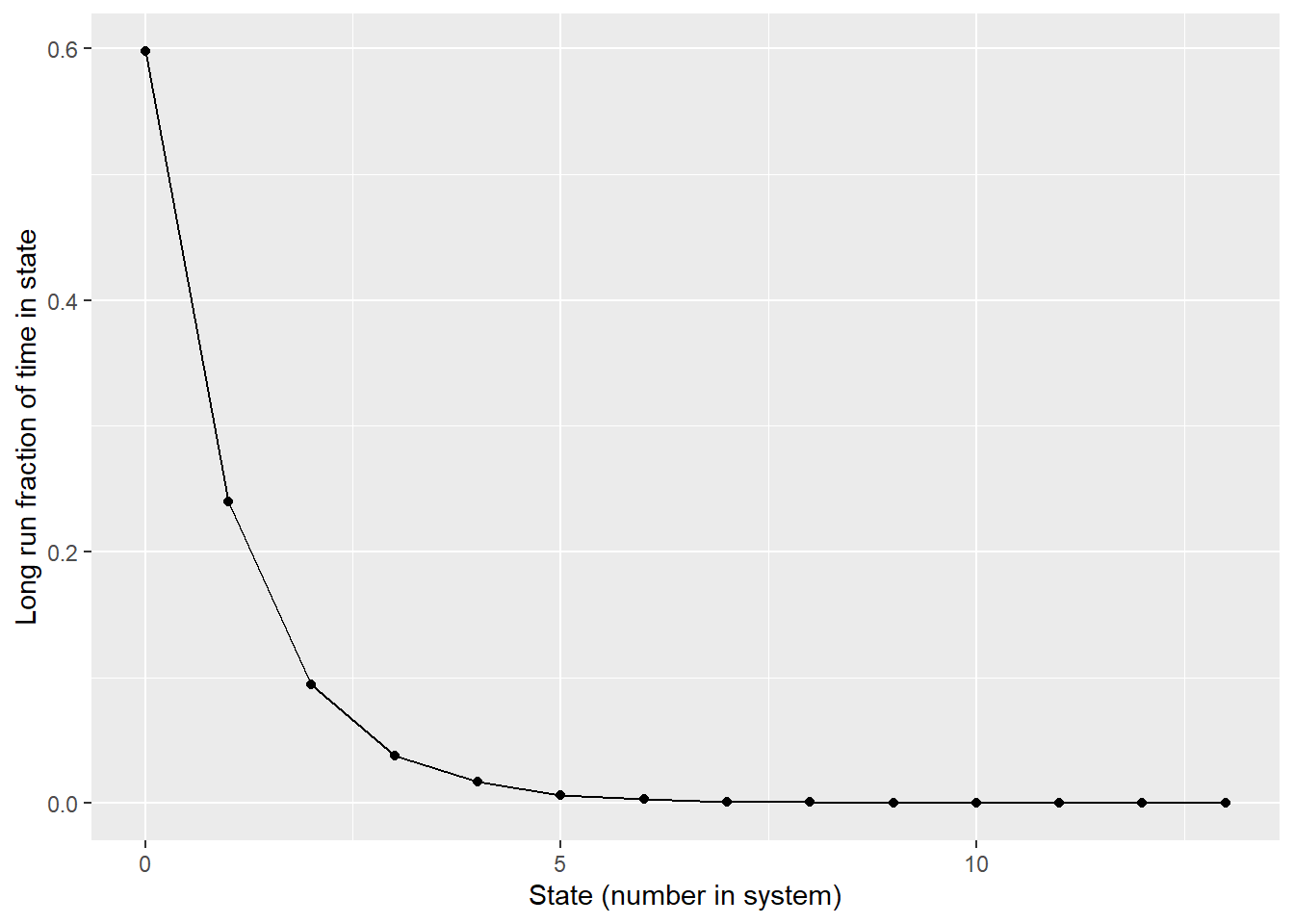

M/M/1 Queue theoretical stationary distribution

lambda = 0.2

mu = 0.5

x = 0:10

px = dgeom(x, 1 - lambda / mu)

stationary_distribution = data.frame(x, px)

stationary_distribution |>
  kbl(digits = 3) |>
  kable_styling()

x	px
0	0.600
1	0.240
2	0.096
3	0.038
4	0.015
5	0.006
6	0.002
7	0.001
8	0.000
9	0.000
10	0.000

stationary_distribution |>
  ggplot(aes(x = x,
             y = px)) +
  geom_point() +
  geom_line() +
  labs(x = "State (number in system)",
       y = "Stationary probability of state")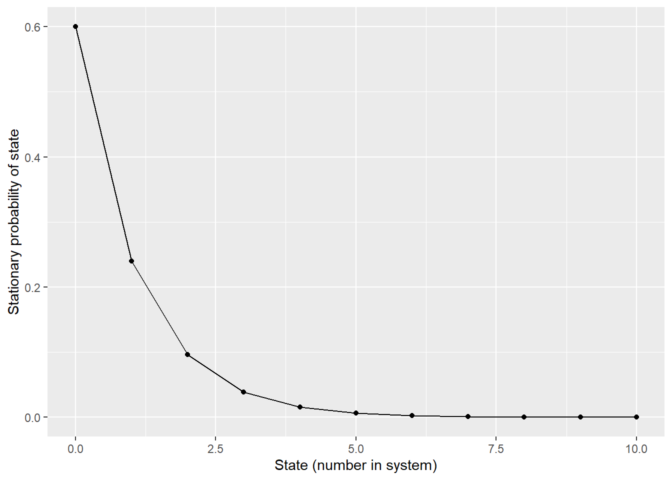

M/M/1 Queue: Mean time until state 4

# Since we want expected time until state 4, treat state 4 as absorbing
# And treat states 0, 1, 2, 3 as transient
# submatrix of transition probability matrix of embedded discrete time chain
# only transition probabilities for "transient" states to "transients" states

QD = rbind(
  c(0, 1, 0, 0),
  c(5, 0, 2, 0) / 7,
  c(0, 5, 0, 2) / 7,
  c(0, 0, 5, 0) / 7
)

# Mean amount of time spent in each state before leaving
inv_lambda = c(1 / 0.2, rep(1 / (0.2 + 0.5), 3))


# Solve system for mean amount of time until state 4
# See end of Handout 23

solve(diag(nrow(QD)) - QD, inv_lambda)

[1] 198.125 193.125 175.625 126.875

M/M/1 Queue: Time until state 4

lambda = 0.2

mu = 0.5

absorbing_state = 4

n_reps = 10000


T_a = rep(NA, n_reps)


for (i in 1:n_reps) {
  x = 0
  t_a = 0
  while(x < absorbing_state) {
    t_a = t_a + rexp(1) / (lambda + (x > 0) * mu)
    x = x + sample(c(-1, 1), 1, prob = c((x > 0) * mu, lambda))
  }
  T_a[i] = t_a
}


hist(T_a)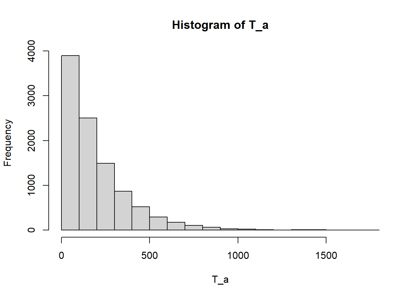

mean(T_a)

[1] 194.5092