library(tidyverse)
library(markovchain) # for plotting state diagram
library(igraph)
library(expm)
library(viridis)
library(viridisLite)
library(ggpubr)
library(grid)
library(gridExtra)
library(prismatic) # for auto-contrast colors (black/numbers number in transition matrix heat map)
library(colourvalues) # for using with viridis
library(kableExtra)Some Functions for Working with Discrete Time Finite State Markov Chains
Disclaimer: these are not the best written or most efficient functions, but they generally do what they’re supposed to do. But there could be some bugs, or some cases that don’t work correctly. In particular, state labels are used inconsistently. And use of color can be improved. Let me know if you have any suggestions or improvements!
Function to simulate a single path of a DTMC
simulate_single_DTMC_path <- function(initial_distribution, transition_matrix, last_time){

  n_states = nrow(transition_matrix) # number of states

  states = 1:n_states # state space

  X = rep(NA, last_time + 1) # state at time n; +1 to include time 0

  X[1] = sample(states, 1, replace = TRUE, prob = initial_distribution) # initial state

  for (n in 2:(last_time + 1)){

    X[n] = sample(states, 1, replace = TRUE, prob = transition_matrix[X[n-1], ])

  }

  return(X)

}
Function to simulate many sample paths of a DTMC (and reshape for plotting)
simulate_DTMC_paths <- function(initial_distribution, transition_matrix, last_time, n_paths = 1) {
  # Columns of output:
  # - n = time (possible values 0:last_time)
  # - path (possible values 1:n_paths)
  # - X = state (possible values 1:n_states); n_states is nrow(P)


  replicate(n_paths, simulate_single_DTMC_path(initial_distribution, transition_matrix, last_time)) |>
    as.data.frame() |>
    mutate(n = 0:last_time) |>
    pivot_longer(cols = !n, names_to = "path", values_to = "X")

}
Function to plot simulated sample paths
plot_DTMC_paths <- function(initial_distribution, transition_matrix, state_names, last_time, n_paths = 1) {

  n_states = nrow(transition_matrix)

  X_df = simulate_DTMC_paths(initial_distribution,
                             transition_matrix,
                             last_time,
                             n_paths)

  if (n_paths > 1) {
    X_df = X_df |>
      # X is jittered vertically; for jitter need continuous X
      # but X needs to be a factor for discrete colors
      mutate(X_jitter = jitter(X),
             n_jitter = jitter(n))
  } else {
    X_df = X_df |>
      mutate(X_jitter = X,
             n_jitter = n)
  }
  alpha_value = min(1, 1 / log10(n_states * n_paths * last_time))

  path_plot <- X_df |>
    ggplot(aes(x = n_jitter,
               y = X_jitter,
               group = path)) +
    geom_point(aes(col = factor(X)),
               alpha = alpha_value) +
    scale_color_viridis(discrete = TRUE,
                        labels = paste(state_names, " (", 1:n_states, ")", sep = ""),
                        guide = guide_legend(reverse = TRUE)) +
    geom_line(col = "gray",
              alpha = alpha_value) +
    scale_x_continuous(breaks = 0:last_time) +
    scale_y_continuous(breaks = 1:n_states) +
    labs(x = "Time (n)",
         y = expression(Value~(X[n])),
         col = "State",
         title = paste(n_paths, "sample paths")) +
    theme_bw() +
    theme(panel.grid.major.y = element_blank(),
          panel.grid.minor.y = element_line(colour = "black"),
          axis.text.x = element_text(angle = 90, size = 8)) +
    # coord_cartesian is for aligning with marginal bar plot
    coord_cartesian(xlim = c(0, last_time))


  path_plot
}
Function to plot simulated marginal distributions
plot_DTMC_simulated_marginal_bars <- function(initial_distribution, transition_matrix, state_names, last_time, n_paths) {
    n_states = nrow(transition_matrix)

    X_df = simulate_DTMC_paths(initial_distribution,
                             transition_matrix,
                             last_time,
                             n_paths)


  dist_plot <- X_df |>
    # X is factor for discrete color fill
    mutate(X = factor(X)) |>
    # Need to reverse order to stack state 1 on bottom
    mutate(X = fct_rev(X)) |>
    group_by(n, X) |>
    tally(name = "freq") |>
    ggplot(aes(x = n,
               y = freq,
               fill = X)) +
    geom_bar(width = 0.5, position = "fill", stat = "identity") +
    scale_fill_viridis(discrete = TRUE,
                       labels = paste(state_names, " (", 1:n_states, ")", sep = ""),
                       # Need to reverse color direction to match the path plot
                       direction = -1) +
    scale_x_continuous(breaks = 0:last_time) +
    scale_y_continuous(expand = c(0, 0)) +
    labs(x = "Time (n)",
         y = "Relative frequency",
         fill = "State",
         title = paste(n_paths, "sample paths")) +
    theme_bw() +
    theme(panel.grid.major = element_blank(),
          panel.grid.minor = element_blank(),
          axis.text.x = element_text(angle = 90, size = 8)) +
    # coord_cartesian is for aligning the two plots
    coord_cartesian(xlim = c(0, last_time))

  dist_plot

}
Function to plot simulated sample paths and simulated marginals
plot_DTMC_simulated_paths_and_marginals <- function(initial_distribution, transition_matrix, state_names, last_time, n_paths) {
  path_plot = plot_DTMC_paths(pi_0, P, state_names, last_time, n_paths)
  marginal_plot = plot_DTMC_simulated_marginal_bars(pi_0, P, state_names, last_time, n_paths)
  path_and_dist_plot <- ggarrange(path_plot +
                                    theme(axis.title.x = element_blank()),
                                  marginal_plot,
                                  ncol = 1,
                                  align = "v",
                                  common.legend = TRUE,
                                  legend = "right")

  path_and_dist_plot

}
Function to plot heat map of transition matrix
shape_transition_matrix_to_plot <- function(P, state_names = NULL) {

  n_states = nrow(P)

  if (is.null(state_names)) state_names = 1:n_states

  as.data.frame.table(t(P), responseName = "transition_probability") |>
    mutate_if(is.factor, as.integer) |>
    rename(after_state = Var1, before_state = Var2) |>
    mutate(after_state = state_names[after_state],
           before_state = state_names[before_state]) |>
    relocate(before_state) |>
    mutate(before_state = factor(before_state),
           after_state = factor(after_state)) |>
    mutate(before_state = fct_rev(before_state))
}
plot_transition_matrix <- function(P, state_names = NULL, n_step = 1) {
n_states = nrow(P)
if (is.null(state_names)) state_names = 1:n_states
P = P %^% n_step
P_plot = shape_transition_matrix_to_plot(P, state_names)
P_plot |>
ggplot(aes(x = after_state,
y = before_state,
fill = transition_probability,
label = sprintf("%0.3f", round(transition_probability, 3)))) +
geom_raster() +
geom_text(aes(color = after_scale(best_contrast(fill,
c("white", "black")))),
show.legend = FALSE) +
scale_fill_viridis(option = "magma",
limits = c(0, 1)) +
scale_x_discrete(expand = c(0, 0),
position = "top") +
scale_y_discrete(expand = c(0, 0)) +
labs(x = "After state",
y = "Before state",
title = paste(n_step, "-step transition matrix", sep =))
}Function to plot spinners for transition matrix
# fix this? Faceting works, except for labels on outside of spinner

plot_transition_spinners <- function(P, n_step = 1) {

  n_states = nrow(P)

  state_color_scale = colour_values(1:n_states,
                                    palette = "viridis")

  spinners = list()

  for (current_start in 1:n_states) {

    p = round((P %^% n_step)[current_start, ], 3)

    df <- data.frame(value = p,
                     group = 1:n_states) |>
      mutate(color = colour_values(group,
                                   palette = "viridis")) |>
      filter(p > 0) |>
      mutate(group = factor(group))

    df2 <- df |>
      mutate(csum = rev(cumsum(rev(value))),
             pos = value / 2 + lead(csum, 1),
             pos = if_else(is.na(pos), value / 2, pos))

    spinner <- ggplot(df, aes(x = "",
                              y = value,
                              fill = group)) +
      geom_col() +
      geom_text(aes(label = value,
                    color = after_scale(best_contrast(fill,
                                                      c("white", "black")))),
                position = position_stack(vjust = 0.5)) +
      coord_polar(theta = "y",
                  direction = -1) +
      scale_fill_manual(values = df$color) +
      scale_y_continuous(breaks = df2$pos,
                         labels = df$group) +
      theme(axis.ticks = element_blank(),
            axis.title = element_blank(),
            axis.text = element_text(size = 10),
            legend.position = "none", # Removes the legend
            panel.background = element_rect(fill = "white")) +
      labs(title = paste("Given state", current_start))

    spinners[[current_start]] = spinner

  }

  # create dummy plot to get legend

  next_state_legend = get_legend(ggplot(data.frame(x = factor(1:n_states)) |>
                                          mutate(x = fct_rev(x)),
                                        aes(x = "",
                                            y = x,
                                            fill = x)) +
                                   geom_bar(width = 0.5, position = "fill", stat = "identity") +
                                   scale_fill_viridis(discrete = TRUE, direction = -1) +
                                   labs(fill = "Next state"))

  grid.arrange(grobs = spinners,
               nrow = trunc(sqrt(n_states)),
               right = next_state_legend,
               top = textGrob(paste(n_step, "-step transition probabilities", sep = ""),
                              gp = gpar(fontsize = 15)))

}
Function to plot marginal distributions
compute_DTMC_marginal_distributions <- function(initial_distribution, transition_matrix, last_time) {

  n_states = nrow(transition_matrix)

  marginal_distribution = matrix(initial_distribution,
                                 byrow = 1,
                                 ncol = n_states)

  time_n_distribution = initial_distribution

  for (n in 1:last_time) {

    time_n_distribution =  time_n_distribution %*% P

    marginal_distribution = rbind(marginal_distribution, time_n_distribution)

  }

  return(marginal_distribution)
  # each row is marginal distribution at a given time
  # first row is time 0 (initial dist)

}
plot_DTMC_marginal_bars <- function(initial_distribution, transition_matrix, state_names = NULL, last_time) {
n_states = nrow(transition_matrix)
if (is.null(state_names)) state_names = 1:n_states
marginal_distribution_df <- compute_DTMC_marginal_distributions(initial_distribution, transition_matrix, last_time) |>
as.data.frame() |>
mutate(n = 0:last_time) |>
pivot_longer(cols = !n, names_to = "state", values_to = "probability") |>
mutate(state = str_remove(state, "V"))
marginal_dist_plot <- marginal_distribution_df |>
mutate(state = fct_rev(state)) |>
ggplot(aes(x = n,
y = probability,
fill = state)) +
geom_bar(width = 0.5, position = "fill", stat = "identity") +
scale_fill_viridis(discrete = TRUE,
labels = paste(state_names, " (", 1:n_states, ")", sep = ""),
direction = -1) +
scale_x_continuous(breaks = 0:last_time) +
scale_y_continuous(expand = c(0, 0)) +
labs(x = "Time (n)",
y = "Probability",
fill = "State",
title = "Marginal distribution at each time") +
theme_bw() +
theme(panel.grid.major = element_blank(),
panel.grid.minor = element_blank(),
axis.text.x = element_text(angle = 90, size = 8)) +
coord_cartesian(xlim = c(0, last_time))
marginal_dist_plot
}Function to plot state diagram
This uses markovchain and igraph.
Need to fix function. Why won’t edge label color match edge color??? Something to do with edge.curved?
plot_state_diagram <- function(transition_matrix, state_names = NULL) {

  n_states = nrow(transition_matrix)

  if (is.null(state_names)) state_names = 1:n_states

  dtmc <- new("markovchain",
              states = as.character(state_names),
              transitionMatrix = P,
              name = "dtmc")

  dtmc_igraph <- as(dtmc, "igraph")

  # to force limits at (0, 1)
  prob_color_scale = data.frame(prob = (0:1000) / 1000,
                                color = colour_values((0:1000) / 1000,
                                                      palette = "magma"))

  prob_color = data.frame(prob = round(E(dtmc_igraph)$prob, 3)) |>
    left_join(prob_color_scale) |>
    pull(color)

  E(dtmc_igraph)$color = prob_color

  edge_attr(dtmc_igraph, "label") <- round(E(dtmc_igraph)$prob, 2)

  plot(dtmc_igraph,
       layout = layout_in_circle,
       edge.curved = 0.2,
       vertex.size = 30,
       vertex.color = colour_values(V(dtmc_igraph)$name, palette = "viridis"),
       vertex.label.color = after_scale(best_contrast(colour_values(V(dtmc_igraph)$name,
                                                                    palette = "viridis"),
                                                      c("white", "black"))),
       edge.color = E(dtmc_igraph)$color,
       #     edge.label.color = prob_color,
       edge.label.color = E(dtmc_igraph)$color,
       edge.arrow.size = 0.5)

}
Function to compute stationary distribution for a finite state, irreducible transition matrix
compute_stationary_distribution <- function(P){

  s = nrow(P)

  rep(1, s) %*% solve(diag(s) - P + matrix(rep(1, s * s), ncol = s))

}
Function to plot proportion of steps in each state for single sample path
plot_sample_path_proportions <- function(initial_distribution, transition_matrix, state_names = NULL, last_time) {

  n_states = nrow(transition_matrix)

  if (is.null(state_names)) state_names = 1:n_states

  X_df = simulate_DTMC_paths(initial_distribution = initial_distribution,
                             transition_matrix = transition_matrix,
                             last_time = last_time,
                             n_paths = 1)

  path_plot <- X_df |>
    ggplot(aes(x = n,
               y = X)) +
    geom_point(aes(col = factor(X))) +
    scale_color_viridis(discrete = TRUE,
                        labels = paste(state_names, " (", 1:n_states, ")", sep = ""),
                        guide = guide_legend(reverse = TRUE)) +
    geom_line(col = "gray",
              alpha = 0.3) +
    scale_y_continuous(breaks = 1:n_states,
                       labels = paste(state_names, " (", 1:n_states, ")", sep = "")) +
    labs(x = "Time (n)",
         y = expression(Value~(X[n])),
         col = "State",
         title = "Title") +
    theme_bw() +
    theme(panel.grid.major.y = element_blank(),
          panel.grid.minor.y = element_line(colour = "black"),
          axis.text.x = element_text(angle = 90, size = 8)) +
    coord_cartesian(xlim = c(0, last_time))


  path_plot_bar <- X_df |>
    mutate(X = factor(X)) |>
    group_by(X) |>
    tally(name = "freq") |>
    mutate(rel_freq = freq / sum(freq)) |>
    ggplot(aes(x = X,
               y = rel_freq,
               fill = X)) +
    geom_col() +
    coord_flip() +
    scale_x_discrete(breaks = 1:n_states,
                       labels = paste(state_names, " (", 1:n_states, ")", sep = "")) +
    scale_fill_viridis(discrete = TRUE,
                       direction = 1,
                       guide = guide_legend(reverse = TRUE)) +
    scale_y_continuous(limits = c(0, 1),
                       expand = c(0, 0)) +
    labs(y = "Relative frequency",
         fill = "State",
         x = "State",
         title = "Title") +
    theme_bw() +
    theme(panel.grid.major = element_blank(),
          panel.grid.minor = element_blank())

  ggarrange(path_plot,
            path_plot_bar,
            ncol = 2,
            legend = "none")
}
Example: Markov’s letters
state_names = c("vowel", "consonant")

P = rbind(
  c(0.1, 0.9),
  c(0.7, 0.3)
)

pi_0 = c(0.5, 0.5)

last_time = 20
Single sample path
plot_DTMC_paths(pi_0, P, state_names, last_time)
Many sample paths
plot_DTMC_paths(pi_0, P, state_names, last_time, n_paths = 100)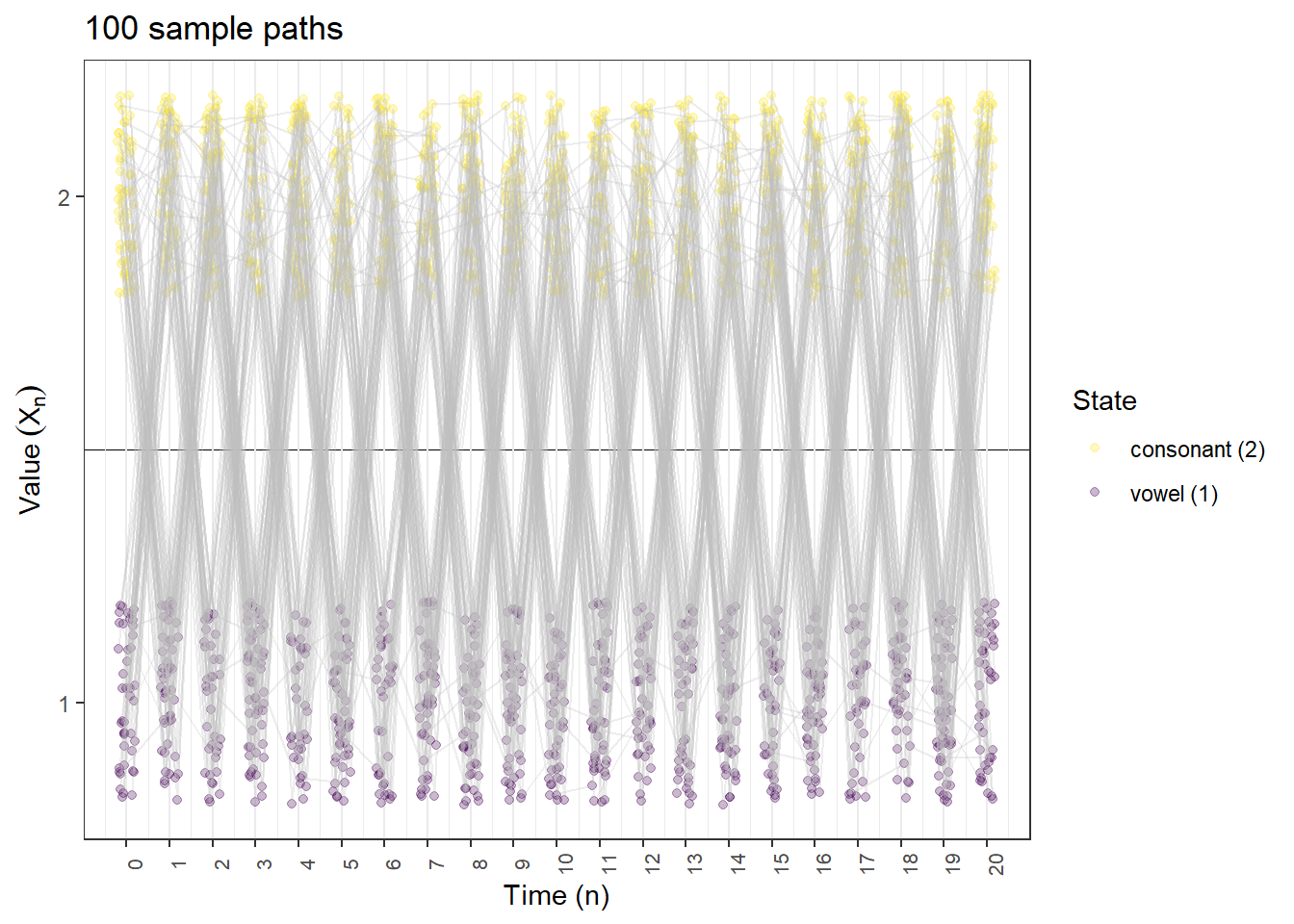
Simulated marginal distributions
plot_DTMC_simulated_marginal_bars(pi_0, P, state_names, last_time, n_paths = 100)
Simulated paths and marginals
plot_DTMC_simulated_paths_and_marginals(pi_0, P, state_names, last_time, n_paths = 100)
Transition matrix
plot_transition_matrix(P, state_names)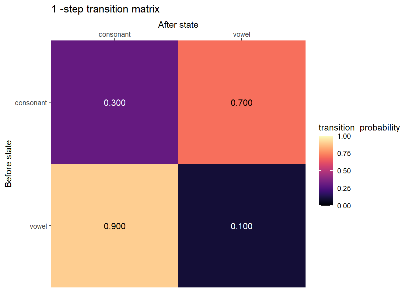
Several step transition matrix
plot_transition_matrix(P, state_names, n_step = 3)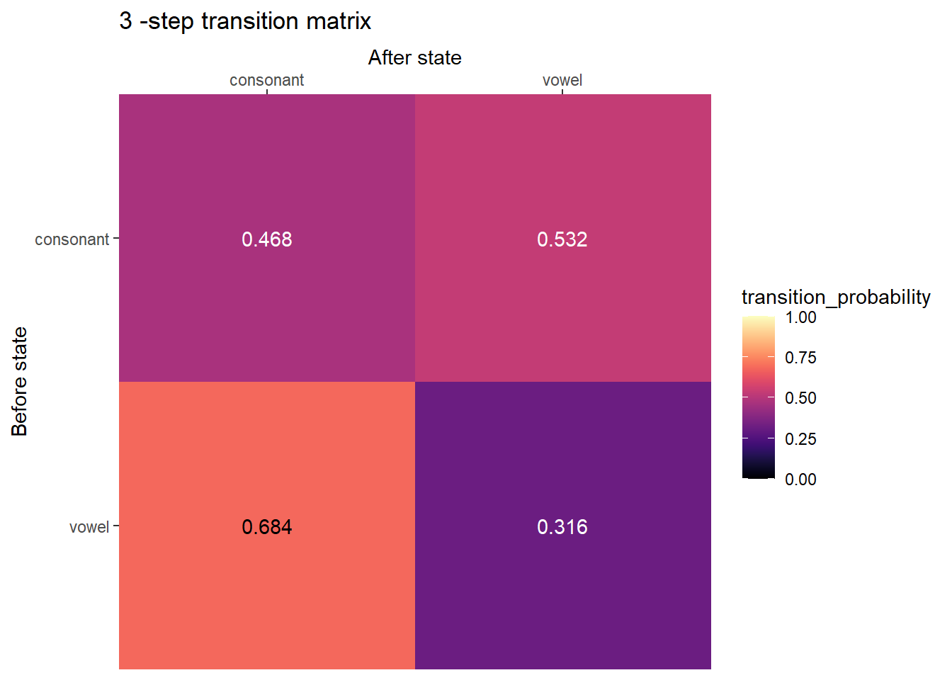
1-step transition spinners
plot_transition_spinners(P)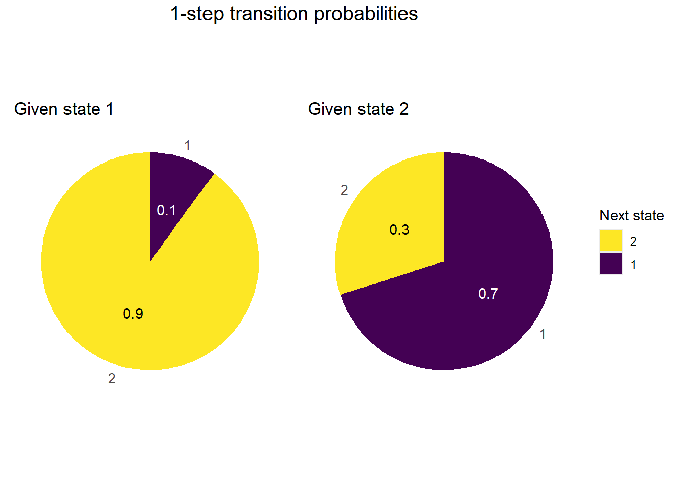
Several-step transition spinners
plot_transition_spinners(P, n_step = 3)
Marginal distributions
plot_DTMC_marginal_bars(pi_0, P, state_names, last_time = 20)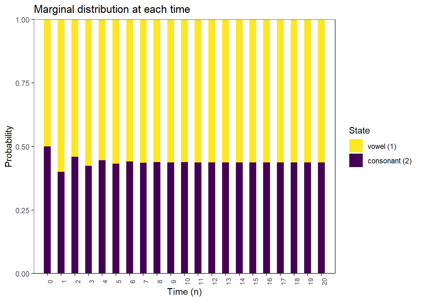
State diagram
plot_state_diagram(P)Joining with `by = join_by(prob)`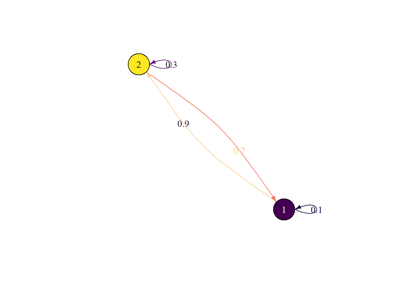
plot_state_diagram(P, state_names)Joining with `by = join_by(prob)`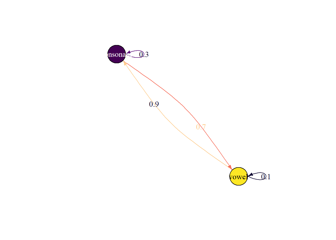
Stationary distribution
compute_stationary_distribution(P) [,1] [,2]
[1,] 0.4375 0.5625First 10 steps: proportion of steps in each state
plot_sample_path_proportions(pi_0, P, state_names, last_time = 10)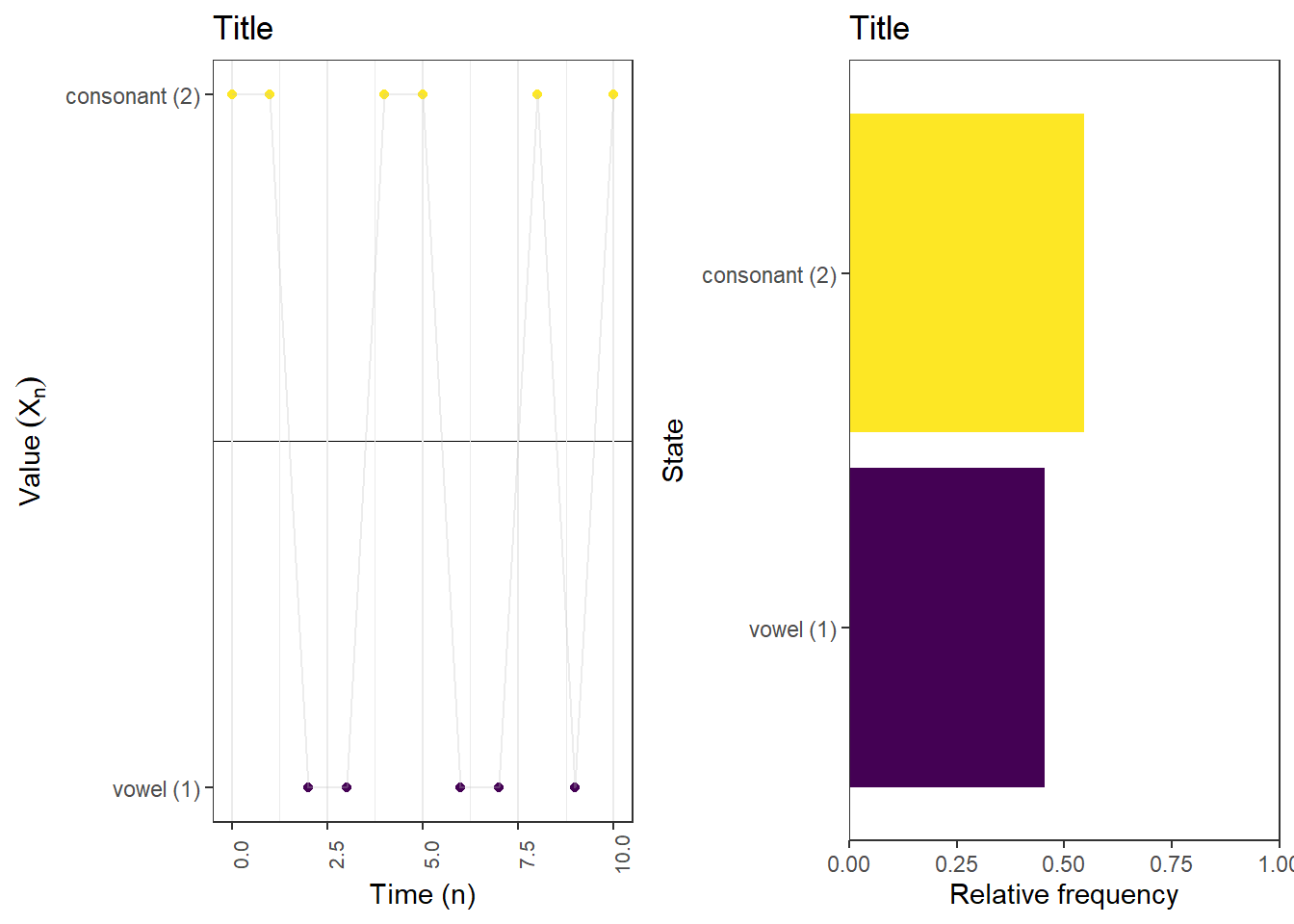
Long run proportion of steps in each state
plot_sample_path_proportions(pi_0, P, state_names, last_time = 1000)