Stationary Distributions and Long Run Behavior of CTMCs

Seagull

Q = rbind(
  c(-1, 0.4, 0.6),
  c(0.8 / 3,  -1 / 3, 0.2 / 3),
  c(0.9 / 5, 0.1 / 5,  -1 / 5)
)

compute_stationary_distribution_ctmc <- function(Q){
  s = nrow(Q)
  Pi = rep(1,s) %*% solve(diag(s) - Q + matrix(rep(1, s * s) - diag(s), ncol = s))
  return(Pi)
}

pi_ctmc = compute_stationary_distribution_ctmc(Q)

pi_ctmc

          [,1]      [,2]      [,3]
[1,] 0.1701389 0.2395833 0.5902778

P = rbind(
  c(0, 0.4, 0.6),
  c(0.8, 0, 0.2),
  c(0.9, 0.1, 0)
)

pi_dtmc = compute_stationary_distribution(P)

pi_dtmc

          [,1]      [,2]      [,3]
[1,] 0.4622642 0.2169811 0.3207547

pi_ctmc = pi_dtmc * 1 / -diag(Q)

pi_ctmc = pi_ctmc / sum(pi_ctmc)

Starting from stationary distribution

library(expm)

pi_ctmc %*% expm(Q * 0.01)

          [,1]      [,2]      [,3]
[1,] 0.1701389 0.2395833 0.5902778

Q = [[-1, 0.4, 0.6],
     [0.8 / 3,  -1 / 3, 0.2 / 3],
     [0.9 / 5, 0.1 / 5,  -1 / 5]]

pi0 = [0.1701389, 0.2395833, 0.5902778]

states = [1, 2, 3]

X = ContinuousTimeMarkovChain(Q, pi0, states)

plt.figure();
X[0.1].sim(10000).plot()
plt.show();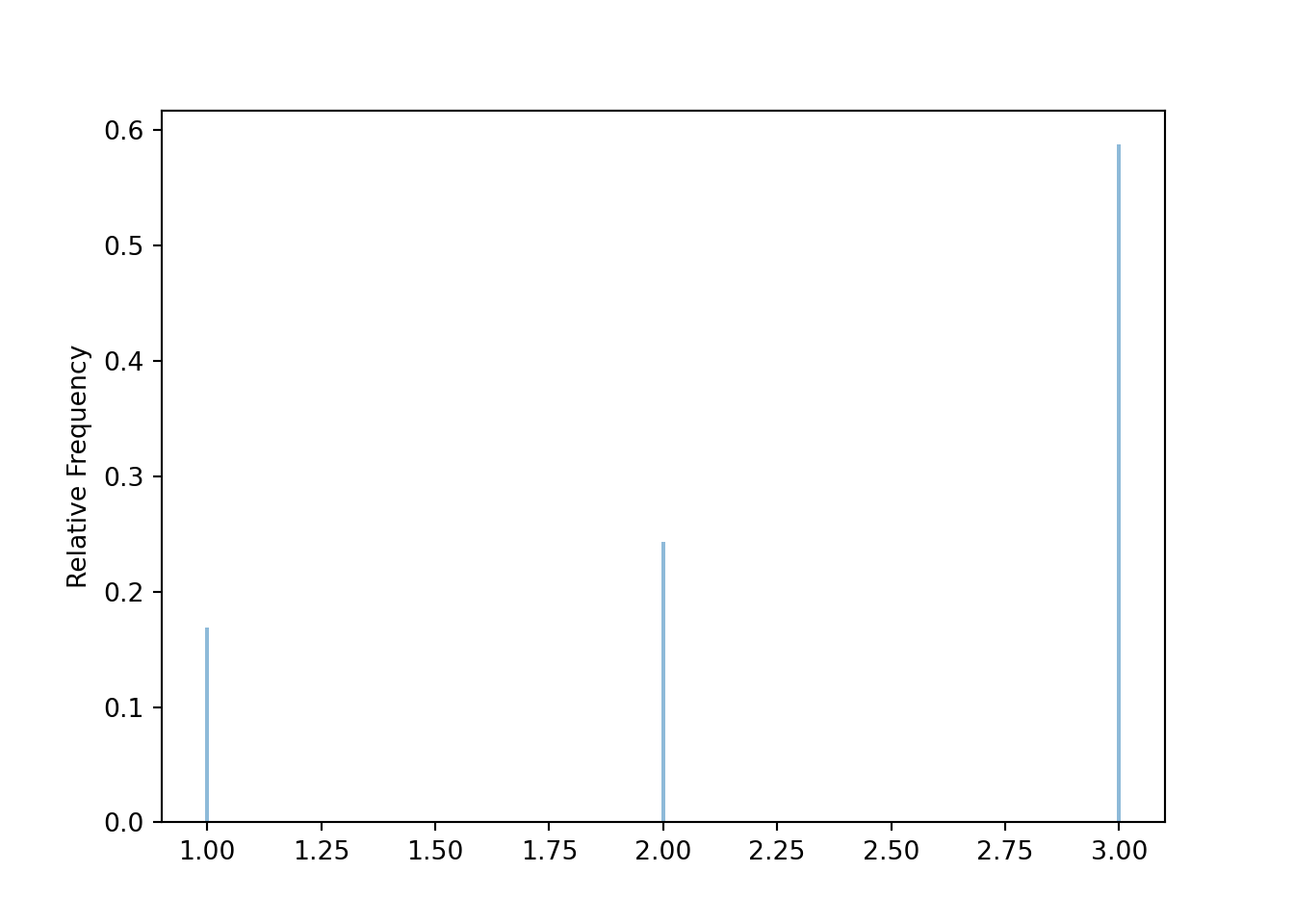

pi_ctmc %*% expm(Q * 0.1)

          [,1]      [,2]      [,3]
[1,] 0.1701389 0.2395833 0.5902778

pi_ctmc %*% expm(Q * 1)

          [,1]      [,2]      [,3]
[1,] 0.1701389 0.2395833 0.5902778

pi_ctmc %*% expm(Q * 10)

          [,1]      [,2]      [,3]
[1,] 0.1701389 0.2395833 0.5902778

Starting from each of the 3 states

expm(Q * 0.01)

            [,1]         [,2]         [,3]
[1,] 0.990060488 0.0039740406 0.0059654717
[2,] 0.002649559 0.9966775877 0.0006728529
[3,] 0.001789509 0.0002030498 0.9980074414

expm(Q * 0.1)

           [,1]        [,2]        [,3]
[1,] 0.90583424 0.037497750 0.056668008
[2,] 0.02501751 0.967728516 0.007253975
[3,] 0.01698773 0.002290251 0.980722020

expm(Q * 1)

          [,1]       [,2]      [,3]
[1,] 0.4208177 0.22068969 0.3584926
[2,] 0.1483652 0.74940800 0.1022268
[3,] 0.1067220 0.03810031 0.8551777

expm(Q * 2)

          [,1]       [,2]      [,3]
[1,] 0.2480892 0.27191543 0.4799953
[2,] 0.1845306 0.59824988 0.2172195
[3,] 0.1418295 0.08468766 0.7734828

expm(Q * 5)

          [,1]      [,2]      [,3]
[1,] 0.1744734 0.2635399 0.5619867
[2,] 0.1832125 0.3755968 0.4411907
[3,] 0.1635832 0.1774727 0.6589441

expm(Q * 10)

          [,1]      [,2]      [,3]
[1,] 0.1706563 0.2447028 0.5846409
[2,] 0.1729511 0.2676561 0.5593928
[3,] 0.1688483 0.2267135 0.6044382

expm(Q * 20)

          [,1]      [,2]      [,3]
[1,] 0.1701608 0.2398022 0.5900369
[2,] 0.1702592 0.2407833 0.5889576
[3,] 0.1700838 0.2390332 0.5908831