Chapter 5 The Normal Model

5.1 Normal Distribution

The normal distribution is the most important probability model in the field of statistics. It is commonly referred to as the so-called bell curve or sometimes as the Gaussian distribution.

It is a continuous probability distribution that is important in the study of probability and statistics for a variety of reasons. First, many natural phenomenon will approximately follow the normal model. Also, many man-made measures, such as standardized test scores, will closely follow the normal distribution.

This distribution is also vital in the theoretical development of many of the methods commonly utilized in applied statistics.

5.2 Normal probability density function

While we will not directly use this formula, the probability density function for the normal distribution is:

\[f(x)=\frac{1}{\sqrt{2\pi \sigma^2}} \exp[-\frac{1}{2}(\frac{(x-\mu)}{\sigma})^2]\] where the parameter $\mu$ is the mean and the parameter $\sigma$ is the standard deviation.

If you have a calculus background, you’ll appreciate not having to evaluate the integral of this function.

5.3 Properties

The normal distribution is a continuous distribution that is:

bell-shaped
unimodal
symmetric
asymptotic
area under the curve is equal to 1

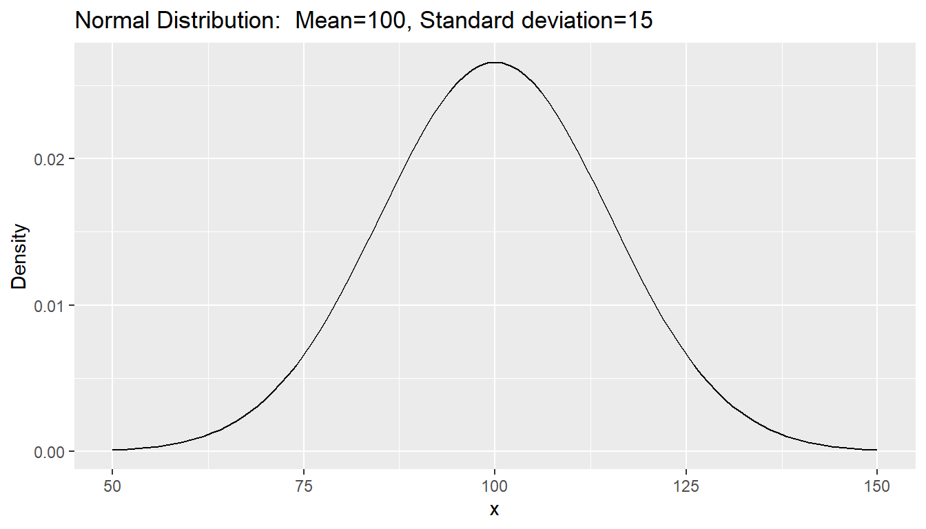
\[X \sim N(100,15)\]

5.4 Standardization

There are an infinite number of normal distribution models, as $\mu$ can take on any real number and $\sigma$ any positive real number. In order to make finding probabilities associated with the normal distribution easier, we generally compute what is known as a , or $z$-score.

The process involves subtracting the mean and dividing by the standard deviation. The resulting $z$-score measures how many standard deviations above or below average a data value is.

\[Z=\frac{X-\mu}{\sigma}\]

Suppose a high school senior takes two mathematics tests, the SAT ($X$) and the ACT ($Y$). Both are normally distributed, but with very different means and standard deviations. If $X \sim N(500,100)$ and $Y \sim N(20,5)$ and the student gets a 640 on the SAT and a 28 on the ACT, then: \[Z_X=\frac{640-500}{100}=1.40\] \[Z_Y=\frac{28-20}{5}=1.60\]

Since the $z$-score is higher for ACT, this student did relatively better on that test than on the ACT.

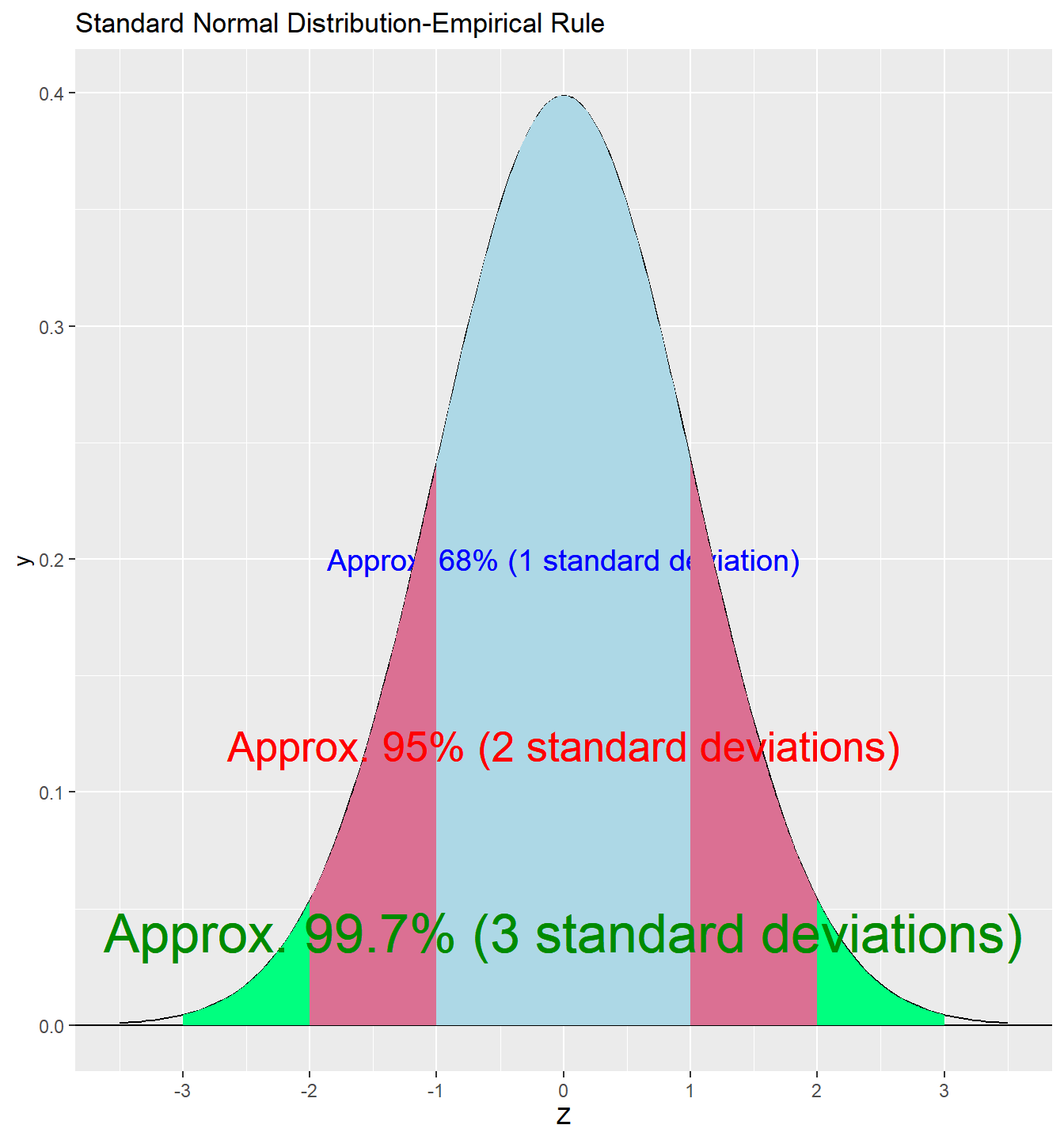
5.5 Empirical Rule

We will get more precise later, but the Empirical Rule tells us that:

about 68% of a normal distribution is within 1 standard deviation of the mean
about 95% of a normal distribution is within 2 standard deviations of the mean
almost the entire curve (99.7%) of the normal distribution is within 3 standard deviations of the mean

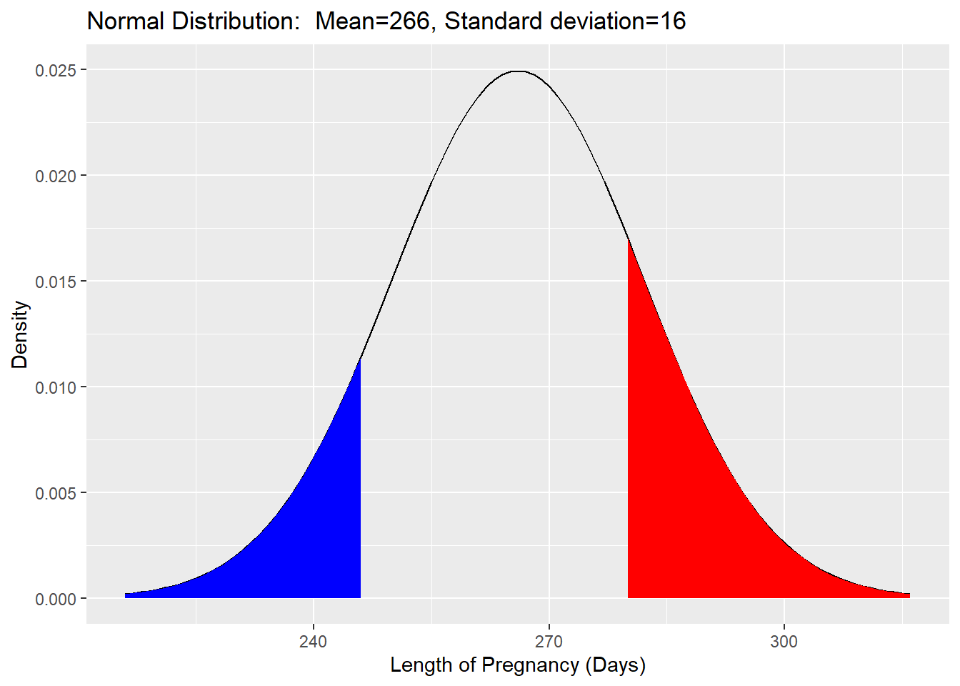
5.6 Normal Probabilities

Assume the mean length of a human pregnancy can be described by a normal distribution with $\mu= 266$ days and $\sigma=16$ days. i.e. $X \sim N(266,16)$. We want to know the probability that a pregnancy lasts less than 246 days, or $P(X<246)$, represented below by the percentage of the area under the curve shaded in blue. Later, we will find $P(X>280)$, which is shaded in red.

5.7 Normal Probability With a Table

We will convert $X=246$ days into a $z$-score.

\[Z=\frac{246-266}{16}=\frac{-20}{16}=-1.25\]

So $P(X<246)=P(Z<-1.25)$. Using the standard normal table, \[P(Z<-1.25)=.1056\]

So a pregnancy lasting 246 days or less happens about 10.56% of the time, or $X=246$ is approximately the 11th percentile of the distribution.

To find $P(X>280)$, first standardize.

\[Z=\frac{280-266}{16}=0.88\]

\[ \begin{aligned} P(X>280)= & P(Z>0.88) \\ = & 1-P(Z<0.88) \\ = & 1-.8106 \\ = & .1894 \\ & \\ P(246<X<280)= & P(-1.25<Z<0.88)\\ = & .8106-.1056 \\ = & .7050\\ \end{aligned} \]

5.8 Normal Probabilities With Technology

With the TI 83/84 calculator, go to 2nd, VARS, and choose Option 2: normalcdf in the DISTR menu. The calculator expects one to enter normalcdf(lower $z$-score, upper $z$-score).

$P(Z<-1.25)=\text{normalcdf(-99999999,-1.25)}=.1056$ (the large negative value is used since the normal curve will stretch on the left to $-\infty$.
$P(Z>0.88)=\text{normalcdf(0.88,99999999)}=.1894$ (the large positive value is used since the normal curve will stretch on the right to $\infty$; the answer is slightly different than the tabled answer because we were forced to round the $z$-score to 2 decimal places when using the table)
$P(-1.25<Z<0.88)=\text{normalcdf(-1.25,0.88)}=.7049$

5.9 Probabilities without Standardizing

With technology, we can find probabilities without standardizing (finding the $z$-score). If we have $X \sim N(180,24)$ and we want $P(X>220)$, you would

\[P(X>220)=\text{normalcdf(220,99999999,180,24)}=.0478\]

5.10 Inverse Normal Problem

In the so-called ‘inverse’ normal problem, we start off knowing the area under the curve (percentile) and we want to find what value of the variable $X$ corresponds to that percentage.

A college will only accept students that score in the top 15% on a standardized test with scores $Y \sim N(\mu=400,\sigma=100)$. John is applying to that score and he wants to know what actual score $Y$ is necessary on the test to qualify.
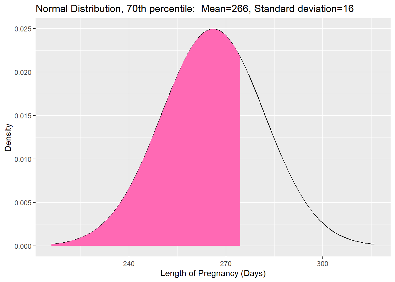
The length of human pregnancies is approx. normal where $X \sim N(266,16)$. Suppose we want to know the 70th percentile of this distribution, or in other words the ‘cut-off’ value separating the shortest 70% of pregnancies from the longest 30%.

5.11 Graph of the Inverse Normal Problem

70th percentile for $X \sim N(266,16)$

5.12 Normal Percentiles With The Table

In order to determine the 70th percentile for human pregnancies using a normal table, we first must determine the $z$-score that corresponds to the 70th percentile.

This is done by looking up an area of .7000 in the ‘middle’ of the normal curve table, and working back to find the row and column to determine the $z$-score.

The closest area to .7000 is .6984, which is on the row for 0.5 and column for 0.02, making the desired standardized score of $Z=0.52$. If you are at the 70th percentile of a normal distribution, you are 0.52 standard deviations above average.

5.13 Use the $z$-score formula

Now that we know the $z$-score for the 70th percentile of a standard normal distribution is $Z=0.52$, and the fact that the distribution of the length of human pregnancies is approx. normal with mean 266 and standard deviation 16, we use the standardization formula to solve for $X$.

\[ \begin{aligned} Z = & \frac{X-\mu}{\sigma} \\ 0.52 = & \frac{X-266}{16} \\ X = & 266+0.52\times 16 \\ X = & 274.32 \\ \end{aligned} \]

5.14 Normal Percentiles With Technology

Let’s find some percentiles with the TI-83/84 calculator.

With the calculator, go to 2nd, VARS, and choose Option 3: invNorm in the DISTR menu. The calculator expects one to enter invNorm(area,mu,sigma).

For the 70th percentile of the pregnancy distribution, enter invNorm(.70,266,16). The answer is 274.39.

For the top 15% of the standardized test score distribution (area below is 85%), where $Y \sim N(400,100)$, use invNorm(.85,400,100). The answer is 503.64.

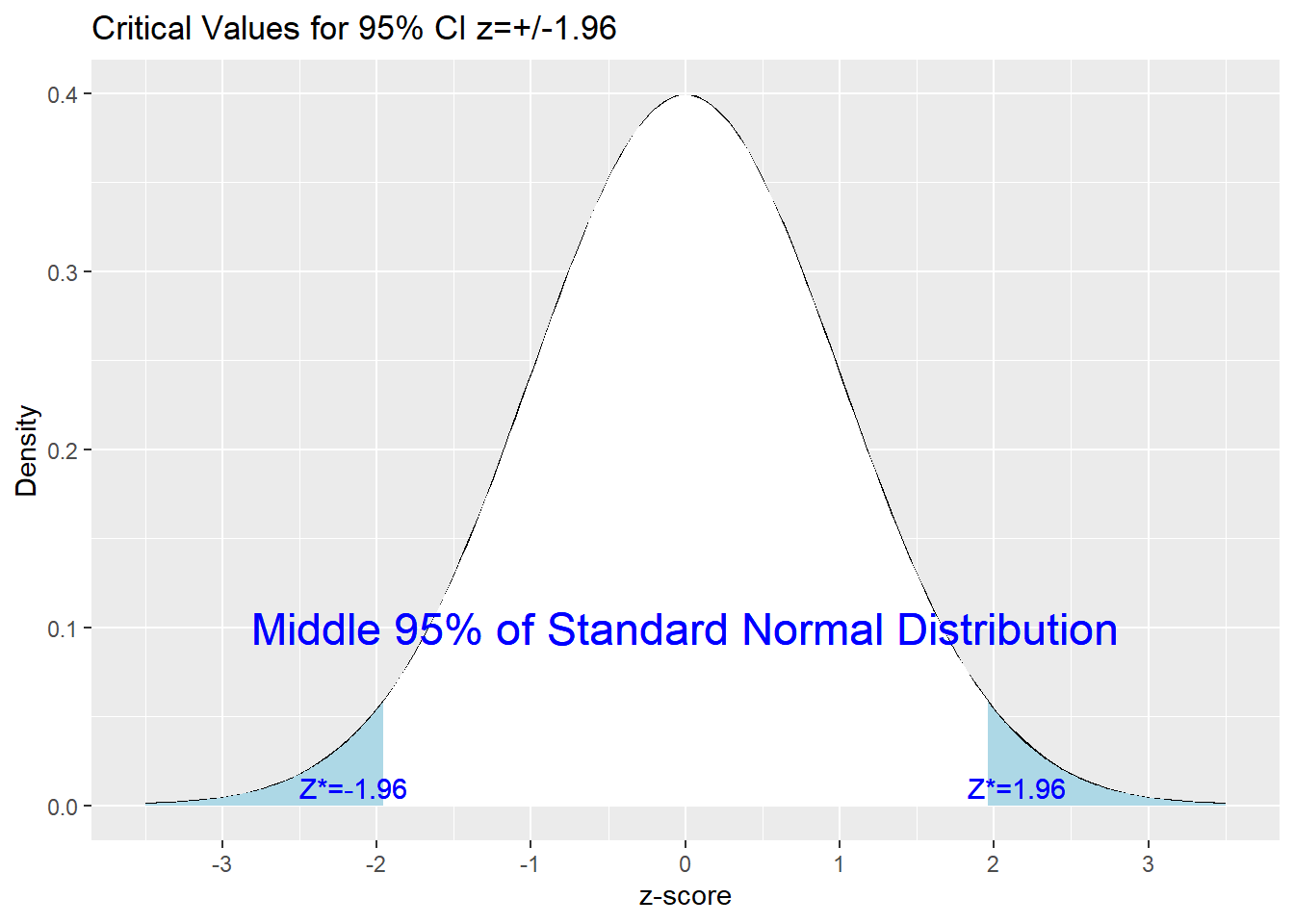
5.15 Middle $100(1-\alpha)$% of the Normal Distribution

Later this semester, when we see how margins of errors for polls and statistical studies are computed, we will see that knowing the $z$-scores that mark off the middle $100(1-\alpha)$% of the standard normal distribution is important.

Let’s let $\alpha=0.05$, so $100(1-.05)=95$%; this is the confidence level that is typically used in finding the margin of error.

We need to divide the $\alpha=0.05$ into two equal pieces to put in the tails of the normal distribution, so $\frac{\alpha}{2}=\frac{0.05}{2}=0.025$. So we can find either the $z$-score that corresponds to an area of 0.0250 the $z$-score that corresponds to an area of 0.9750.

For 95% confidence, the critical value is $z=\pm 1.96$. This is more precise that the approximately 2 standard deviations that we get from the Empirical Rule. You can this either from the table or by using invNorm(.025) and invNorm(.975) on your calculator.

The blue tails in the graph below each have area=$\alpha/2=.025$ and the white area between is equal to 0.95.

STA 135 Notes (Murray State)