Chapter 7 Simple Linear Regression
7.1 Finding the Least Squares Regression Model
Data Set:
Variable \(X\) is Mileage of a used Honda Accord (measured in thousands of miles); the \(X\) variable will be referred to as the explanatory variable, predictor variable, or independent variable
Variable \(Y\) is Price of the car, in thousands of dollars. The \(Y\) variable will be referred to as the response variable or dependent variable
Before we even collect some data, compute statistics and construct a scatterplot, what would you expect to be true about the strength and the direction of the correlation between Mileage and Price?
In statistics, we often want to know if two variables \(X\) and \(Y\) are mathematically related to each other, and eventually if we can form a mathematical model to explain or predict variable \(Y\) based on variable \(X\). In a high school or college algebra class, you might have called this the line of best fit. I will refer to it as the simple linear regression model or the least squares regression model.
This is a random sample of \(n=10\) used Honda Accords. I have computed the means and standard deviations of both variables, along with the correlation.
| \(X\) | \(Y\) |
|---|---|
| 74.9 | 12.0 |
| 53.0 | 17.9 |
| 79.1 | 15.7 |
| 50.1 | 12.5 |
| 62.0 | 9.5 |
| 4.8 | 21.5 |
| 89.4 | 33.5 |
| 20.8 | 22.8 |
| 4.8 | 26.8 |
| 48.3 | 13.6 |
## [1] "Variable X (Mileage)"## mean sd
## 48.72 29.99521## [1] "Variable Y (Price)"## mean sd
## 18.58 7.548186## [1] "Correlation between X and Y"## [1] -0.1912Does the value of the correlation coefficient surprise you, in either the strength and/or direction of hte correlation?
7.2 Guess The Line of Best Fit
Below is a scatterplot where we are attempting to “guess” the line of best fit.
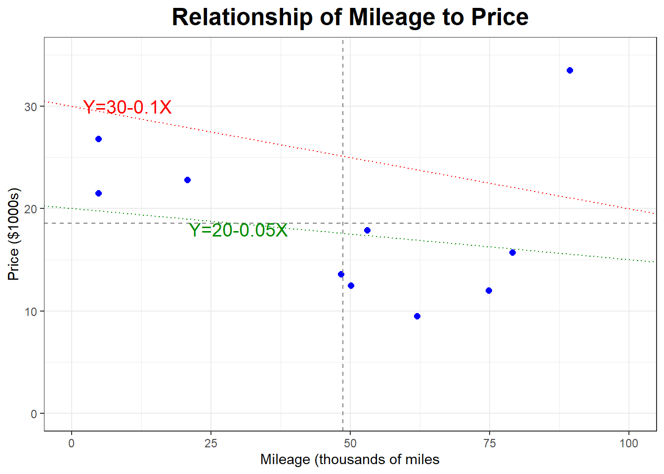
Which of these lines do you think is “better” for fitting our points? Are there any points (cars) that seem to not fit the general linear trend? If so, what’s the reason for it?
You might have noticed that one of the cars (Car #7) has Mileage \(X=89.4\) (the highest mileage car in the sample) but a Price \(Y=33.5\) (the highest price in the sample). Does this seem right?
For now, we will go ahead and leave Car #7 as is, and revisit that point later, as it might be an outlier or an influential point in our linear regression model.
7.3 Least Squares Method
Obviously we aren’t going to actually find the equation for a statistical model by guessing and using trial and error. We need to have some sort of mathematical method of selecting and computing the equation of the “line of best fit”.
The equation of this line will be \[\hat{Y}= b_0 + b_1 X\] Many books use \(a\) and \(b\) instead.
\[\hat{Y} = a + b X\]
Sometimes we just use the actual names of the variables. \[\hat{Price} = b_0 + b_1 \times Mileage\]
\(X\) is the value of our explanatory or independent variable (the Mileage of the used caT in this example)
\(\hat{Y}\) (“y-hat”) is the predicted value of our response or dependent variable (predicted Price in this case). Suppose you have a Honda Accord with 40,000 miles (\(X=40\)) that you want to sell; we could use the regression model to predict its Price, and denote this prediction with \(\hat{Y}\). When you actually sell the car, the actual Price will be \(Y\) (without the hat).
\(b_1\) is the slope of the regression line and \(b_0\) is the \(y\)-intercept of the line. You probably used \[y=mx+b\] in high school with \(m\) for slope and \(b\) for the \(y\)-intercept. Statisticians never use \(m\) to represent the slope; we prefer \(b_1\) and the parameters would be \(\beta_0\) and \(\beta_1\) if we had data for the entire population of used Honda Accords.
In order to estimate the numerical values of the slope and intercept \(b_1\) and \(b_0\), we use a mathematical criterion called least squares estimation. We choose the line whose equation will minimize the sum of squared residuals.
\[SSResiduals =\sum_{i=1}^n (Y_i - \hat{Y}_i)^2 = \sum_{i=1}^n e_i^2\]
What’s a residual? A residual is the vertical distance between an actual observed data point and the predicted point. You can think of it as the “error” in our prediction, and we use the letter \(e\) for it.
\[e=Y-\hat{Y}\]
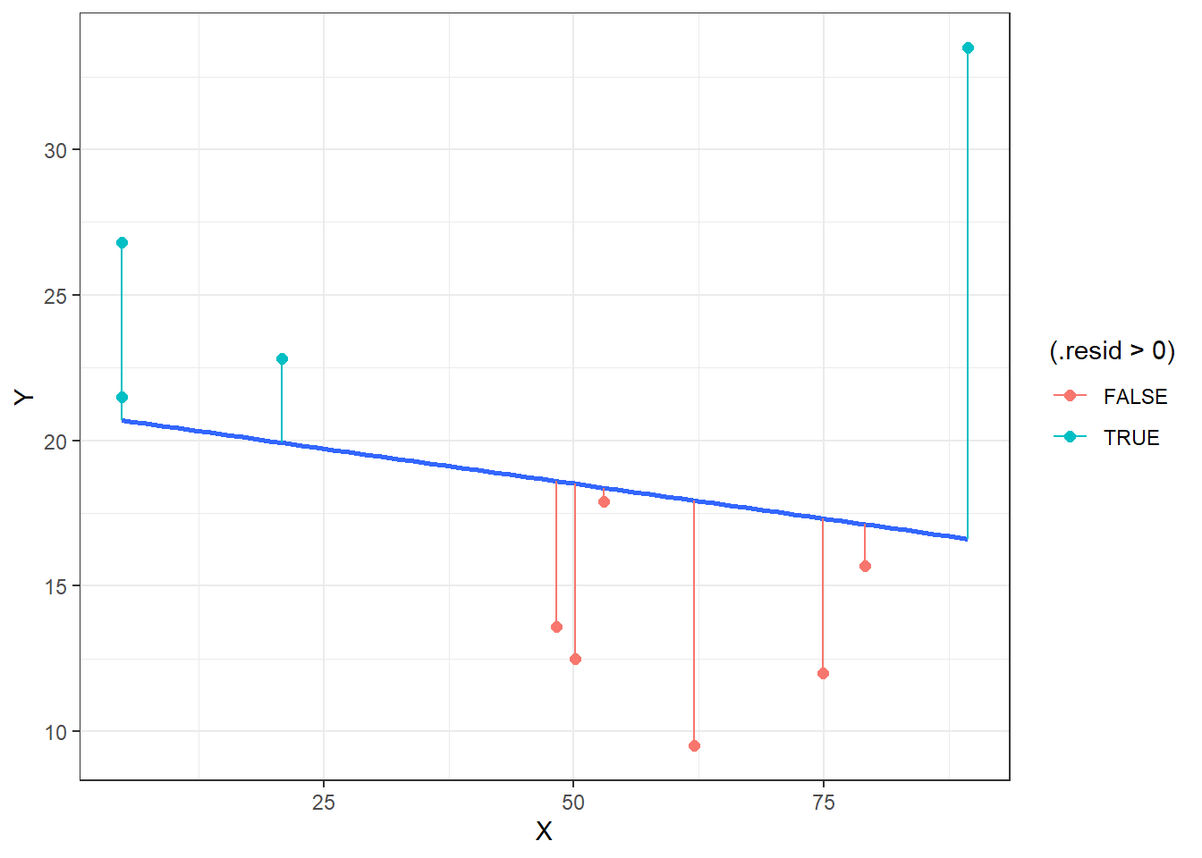
The largest positive residual was for car #7 (\(X=89.4,Y=33.5\)). This is the point the furtherest above the blue least squares regression line, as this car sold (?) for much more than the regression model predicted.
On the other hand, car #5 (\(X=62.0,Y=9.5\)) had the largest negative residual. This car sold for thousands of dollars less than predicted. We could think of some possible reasons why this might be thecase.
Some students have points very close to the line. These residuals are equal to almost zero, indicating that the Price \(Y\) and the predicted Price \(\hat{Y}\) are very close.
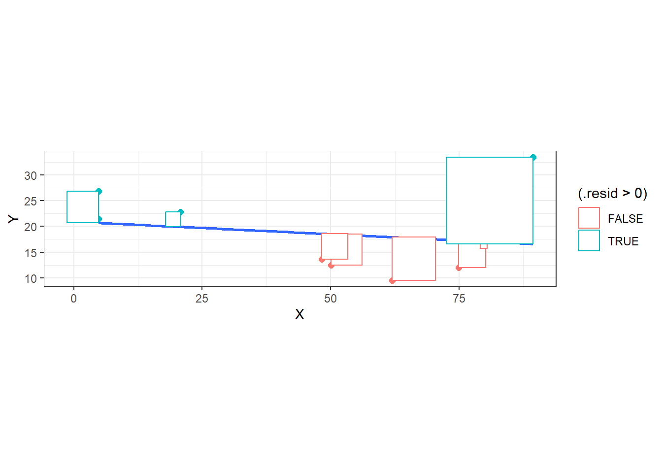
If we square and sum the residuals for all points, we obtain the sum of squared residuals \[SSR = \sum_{i=1}^n (Y_i - \hat{Y_i})^2\]
The blue least squares regression line is the one that minimizes \(SSR\), represented below as the area of the rectangles. No other line would make the area of those rectangles smaller.
Through the use of calculus, the equations for the least squares regression line are: \[b_1 = r \frac{s_Y}{s_X}\]
\[b_0 = \bar{Y} - b \bar{X}\]
For the used cars example, we get:
\[b_1 = -0.1912 \times \frac{7.5482}{29.9952} = -0.0481\]
\[b_0 = 18.58 - (-0.0481) \times 48.72 = 20.9234\]
Thus, the least squares regression model has the following equation:
\[\hat{Y}=20.9234-0.0481 X\]
7.4 Interpretation of the Regression Model
What do the numerical values of \(b_0\) and \(b_1\) physically represent?
\(b_0\) is the \(y\)-intercept, the predicted value of \(Y\) when \(X=0\). In our case, our model predicts a Price of the car when the Mileage is 0. None of our data had Mileage this low and this is likely less than we would be able to buy a new car for from the Honda dealer.
It is pretty common for the \(y\)-intercept \(b_0\) to have no physical meaning; this happens when \(X\) will never be equal to 0. If we were trying to predict the gas mileage of a car based on its weight, no car weighs \(X=0\) pounds. However, if we are trying to predict the ozone level based on wind speed, a day with no wind would have \(X=0\), and in that case the intercept of the regression equation is the predicted ozone level on a day with no wind.
\(b_1\) is the slope, or the rate of change. It tells us the predicted increase/decrease in \(Y\) with a one unit increase in \(X\). Note that the slope of the regression equation will always have the same sign as the correlation between \(X\) and \(Y\). In our example, \(b_1=-0.0481\) means that we predict the Price will decrease by -0.0481 thousand dollars (or about 48 dollars) for every increase of 1 (one thousand miles) in the Mileage.
7.5 Prediction With The Regression Model
Suppose we try to predict the Price of your used Honda Accord with 40,000 miles, or \(X=40\).
\[\hat{Y} = 20.9234 - 0.0481 \times 40= 18.9994\] This is about $19,000.
Car #7 in our data set has Mileage \(X=89.4\) but had a high Price of \(Y=33.5\). This was the point in the upper right hand corner of the scatterplot that seems to be an outlier or what is called an influential point. It has a large residual.
\[\hat{Y} = 20.9234 - 0.0481 \times 89.4 = 16.3\]
\[e = Y - \hat{Y} = 33.5 - 16.3 = 17.2\]
This car sold for $17,200 more than predicted. How could this happen? Maybe (as was speculated in class) this is a collector’s car or something is “special” about it to warrant such a high price. Often, when we find large residuals, these are sometimes just data entry errors, and by looking at the plot, we can find these mistakes and correct them.
Car #2 had Mileage of \(x=53.0\) and a Price \(Y=17.9\). This is the point on the scatterplot that is the closest to the line, and the residual is close to zero. (The actual price was about $500 less than predicted).
\[\hat{Y} = 20.9234 - 0.0481 \times 53.0 = 18.4\]
\[e = 17.9 - 18.4 = -0.5\]
The coefficient of determination, or \(r^2\), is used as a measure of the quality of a regression model. One reason for using this statistic is that the correlation \(r\) is NOT a percentage, but $r^2 is.
\[r^2=(-0.1912)^2=.037\]
The interpretation of \(r^2\) in our example is: About 3.7% of the variation in the Price of the used Honda Accord is accounted for by the regression model based on Mileage.
As you can see, this result is not terribly impressive, as we want \(r^2\) to be close to 1 (100%).
Suppose that we discover that no one actually bought Car #7 (the car with high mileage being listed at $33,500).
If we delete Car #7 (the influential point), we have a substantial change in the correlation & regression statistics.
## [1] "Mean and Standard Deviation of X, Mileage"## mean sd
## 44.2 27.97025## [1] "Mean and Standard Devaition of Y, Price"## mean sd
## 16.92222 5.76016## [1] "Correlation between Mileage and Price"## [1] -0.8256## [1] "Intercept and Slope"## (Intercept) X
## 24.4369595 -0.1700167## `geom_smooth()` using formula = 'y ~ x'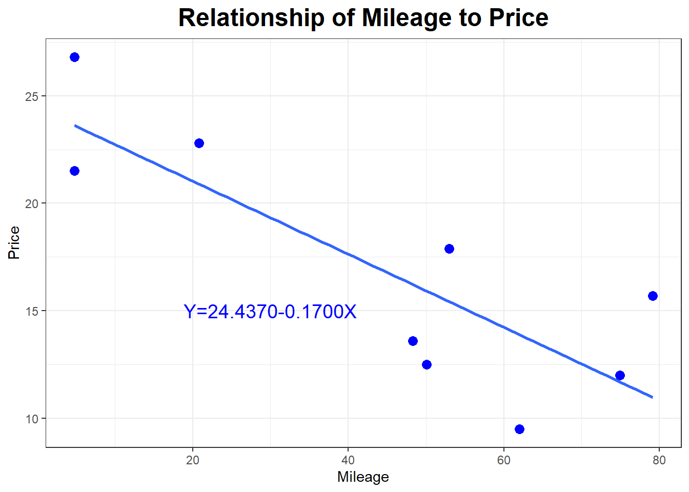
Now the regression model is \[\hat{Y}= 24.437 - 0.17 X\]
with \(r=-0.8256\) (the expected strong negative correlation) and \(r^2=.682\), indicating that about 68.2% of the variation in Price is explained by the model using Mileage.
7.6 Finding The Regression Model With Summary Statistics
Suppose we are looking at the relationship between the Fat (grams) and Calories in a sample of \(n=7\) different fast-food burgers. We have the scatterplot and the summary statistics (means, standard deviations, correlation) but not the original data.
## [1] "Mean and Standard Deviation of X, Fat"## mean sd
## 34.28571 7.80415## [1] "Mean and Standard Devaition of Y, Calories"## mean sd
## 590 89.81462## [1] "Correlation between Mileage and Price"## [1] 0.9606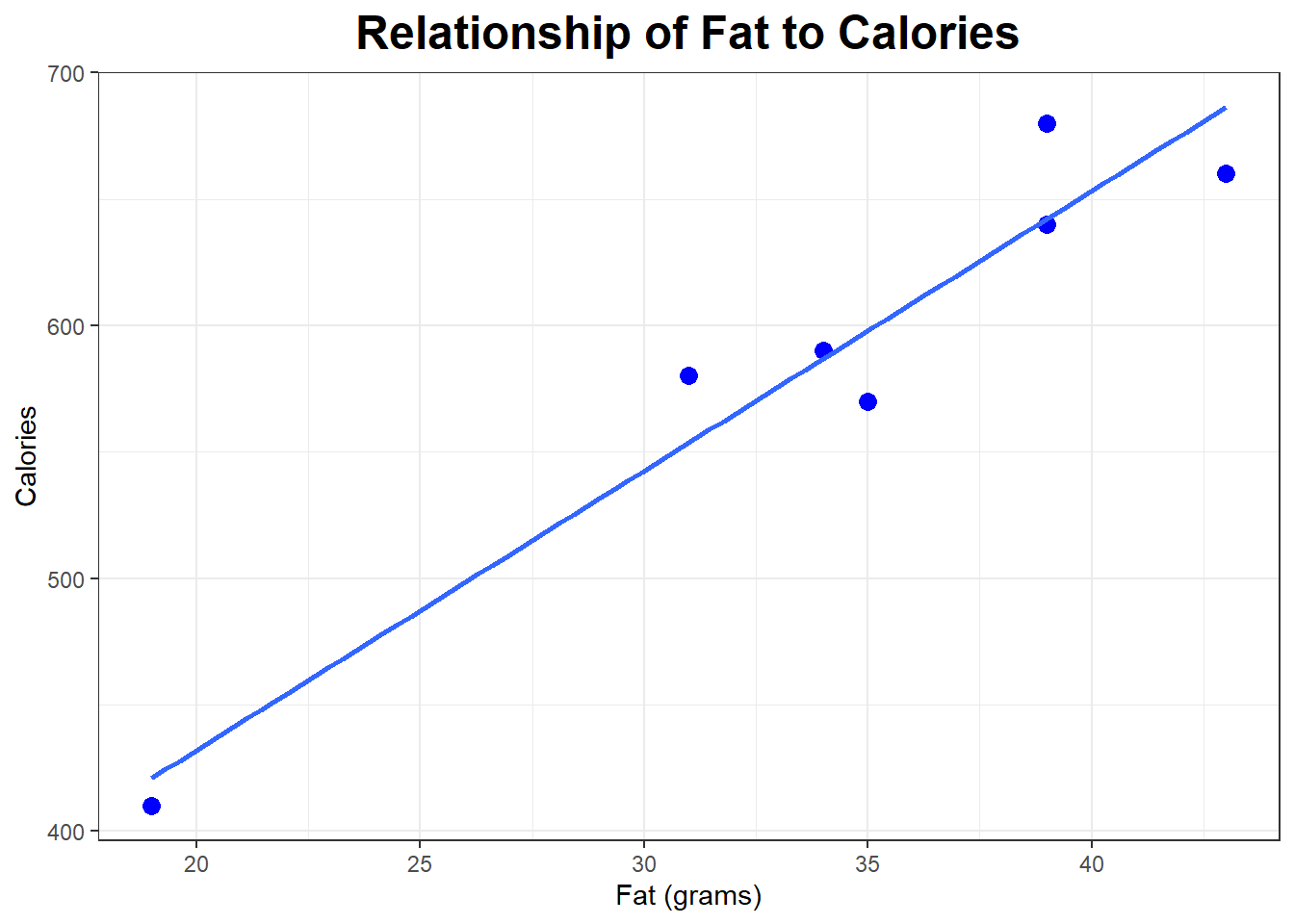
Let’s find the equation of the least squares regression line, and then use it to make a prediction for a couple of burgers that were not part of the original data set.
\[b_1 = r \frac{s_y}{s_x} = 0.9606 \frac{89.8146}{7.8042} = 11.0551\]
\[b_0 = \bar{y} - b_1 \bar{x} = 590 - 11.0551 \times 34.2857 = 210.9682 \]
\[\hat{Y} = 210.9682 + 11.0551 X\]
\[\hat{Calories} = 210.9682 + 11.0551 Fat\]
So, a burger with 0 grams of fat (I don’t think such a burger exists) would be predicted to have about 211 calories, and every increase of 1 gram of fat leads us to predict that it will have about 11 more calories.
A few years ago, Wendy’s introduced a burger called the Baconator Double (intended for people that probably don’t care about calories) that had Fat of \(X=63\) grams. We can make a prediction with our regression model, although none of the burgers in the data set had more than \(X=43\) grams of fat, so we are going beyond the range of regression or extrapolating, so the results can be questionable.
\[\hat{Y} = 210.9682 + 11.0551 \times 63 \approx 907\]
Wow, the predicted or fitted value \(\hat{Y}\) for the Baconator Double is over 900 calories (680 calories was the most in the original data set). The residual is \[e = Y - \hat{Y} = 970 - 907 = 63\] The actual Wendy’s Baconator Double has even more calories (63) than our model predicted!
The \(r^2\) for our burger model is \[r^2=.9606^2=.9228\]
About 92% of the varation in calories in fast-food hamburgers is accounted for by the fat content of that burger.
Here’s another regression model, this one is for \(n=11\) different fast-food chicken sandwiches where \(r=0.947, \bar{x}=20.6, s_x=9.8, \bar{y}=472.7, s_y=144.2\) (I’m not showing the scatterplot there, but it is a strong positive linear trend)
\[\hat{Y} = 185.6514 + 13.9344X\]
\[r^2=(0.947)^2 = 0.897\]
So I have a model for hamburgers and a somewhat different model for chicken sandwiches.
Hardee’s has a Turkey Burger with \(X=17\) grams of fat. If we wanted to predict its calories, which model would you use? (sorry, I don’t have enough data to provide you with a “turkey burger” model)
\[\text{Hamburger Model: } \hat{Y} = 210.9682 + 11.0551 \times 17 \approx 399\]
\[\text{Chicken Sandwich Model: } \hat{Y} = 185.6514 + 13.9344 \times 17 \approx 423\]
So the prediction is a bit higher if we treat the turkey burger as being like a chicken sandwich rather than like a beef burger.
It turns out that the Hardee’s Turkey Burger has \(Y=480\) calories, so both models underpredict and both models would have a positive residual. The chicken sandwich model was closer.
\[\text{Hamburger Model: } e = 480 - 399 = 81\]
\[\text{Chicken Sandwich Model: } e = 480 - 423 = 57\]