Chapter 21 Paired Samples and Blocks
21.1 Paired Samples
Here, we will cover how to test a hypothesis involving paired samples (also called dependent samples or matched pairs). This is when we take two measurements on the same individual and wish to see if some sort of significant change has occurred. Common scenarios include pre-test vs post-test, before vs after, etc. Notice we are not comparing two independent groups (such as comparing a treatment group with a control group); this is a two-sample t-test which we’ll discuss later.
21.2 Hypothesis Test
The paired samples t-test really is just a special kind of one-sample t-test, where we will compute a difference score \(d=y-x\) and perform the t-test (or compute a confidence interval) on the differences \(d\). This is the most basic kind of repeated measures analysis; more advanced methods that won’t be considered in this class include repeated measures ANOVA and multilevel models (also called linear mixed models).
Usually the null value will be zero (although it doesn’t have to be) and it is quite common to use one-sided/directional alternative hypotheses. For example, if I gave a class a pre-test at the beginning of the semester to see what you knew about statistics and a post-test at the end of the semester, I would hope that the mean of the post-test scores are significantly higher than the pre-test scores. If a group of overweight people were going on a diet to try and lose weight, we would expect their weight after the diet to be significantly less than before the diet.
EXAMPLE
An experiment is being conducted to see if one’s reaction time is affected by drinking alcohol. A random sample of \(n=10\) people are tested, with their reaction time measured both before (\(X\)) and after (\(Y\)) consuming alcohol. Suppose we expect that the reaction time will be significantly higher after drinking alcohol, indicating a slowed reaction.
Before doing the paired-samples t-test, I’m going to compute some basic statistics, and review computing the sample variance and standard deviation in a step-by-step process (as you might need to do this on the final exam).
Note that \(\bar{d}=0.09\). This is the mean difference in means; the average subject had a reaction time that was 0.09 seconds slower after drinking alcohol. Notice subjects 5 and 7 have negative differences, as they actually had a faster reaction time after drinking, the opposite of what was expected. This would be like if you did worse on the post-test or if a dieter actually gains weight on the diet.
| Subject | \(x\) (Before) | \(y\) (After) | \(d=y-x\) | \(d-\bar{d}\) | \((d-\bar{d})^2\) |
|---|---|---|---|---|---|
| 1 | 0.40 | 0.56 | 0.16 | 0.07 | 0.0049 |
| 2 | 0.50 | 0.50 | 0.00 | -0.09 | 0.0081 |
| 3 | 0.65 | 0.78 | 0.13 | 0.04 | 0.0016 |
| 4 | 0.45 | 0.67 | 0.22 | 0.13 | 0.0169 |
| 5 | 0.60 | 0.50 | -0.10 | -0.19 | 0.0361 |
| 6 | 0.44 | 0.54 | 0.10 | 0.01 | 0.0001 |
| 7 | 0.60 | 0.55 | -0.05 | -0.14 | 0.0196 |
| 8 | 0.50 | 0.70 | 0.20 | 0.11 | 0.0121 |
| 9 | 0.65 | 0.82 | 0.17 | 0.08 | 0.0064 |
| 10 | 0.45 | 0.52 | 0.07 | -0.02 | 0.0004 |
Notice that \[\bar{d}=\frac{\sum d}{n}=\frac{0.90}{10}=0.09\]
\[s_d^2=\frac{\sum(d-\bar{d})^2}{n-1}=\frac{0.1062}{10-1}=0.0118\] \[s_d=\sqrt{0.0118}=0.1086\]
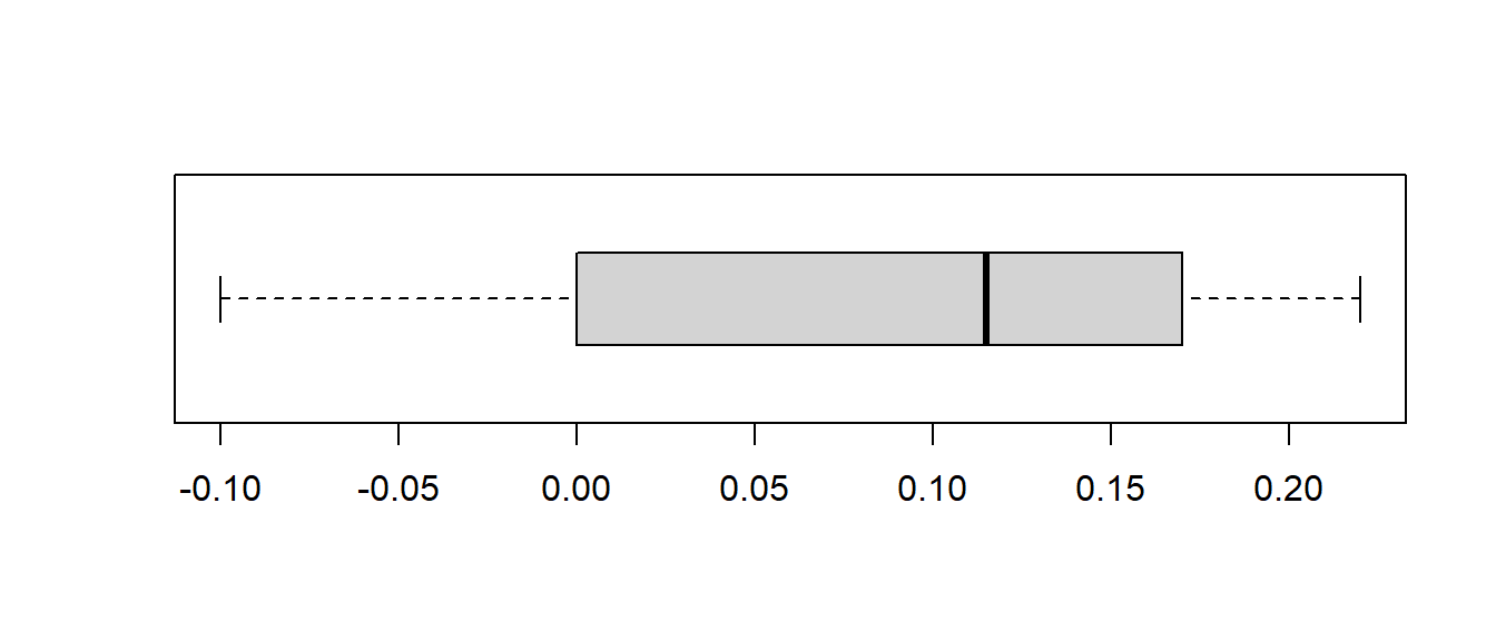
I will also double-check to make sure that the distribution of those differences \(D\) is “nearly normal” and doesn’t contain any outliers with an informal outlier check.
\[Min=-0.10, Q1=0, M=0.115, Q3=0.17, Max=0.22\]
\[IQR=0.17-0=0.17, Step=1.5 \times IQR=0.255\]
\[Q1-Step=0-0.255=-0.255, Q3+Step=0.17+0.255=0.425\]
There are no outliers. I will proceed with the \(t\)-test. What are called non-parametric tests are often used if there are outliers present that can’t be removed from the data; examples include the Wilcoxon Signed Rank Test and the Mann-Whitney Test (we will not study the formulas for these tests).
Step One: Write Hypotheses
\[H_O: \mu_D=0\] \[H_A: \mu_D >0\]
Step Two: Choose Level of Significance
Let \(\alpha=0.05\)
Step Three: Choose Test & Check Assumptions I am satisfied that we have a sample that is random, paired, with the difference satisfying the “nearly normal” condition, so I will use the paired samples t-test.
Step Four: Calculate the Test Statistic
\[t=\frac{\bar{d}-\mu_0}{s_d/\sqrt{n}}\] \[t = \frac{0.09 - 0}{0.1086/\sqrt{10}}\]
\[t = \frac{0.09}{0.0343}\]
\[t=2.620\]
\[df=n-1=9\]
Step Five: Make a Statistical Decision (via the \(p\)-value)
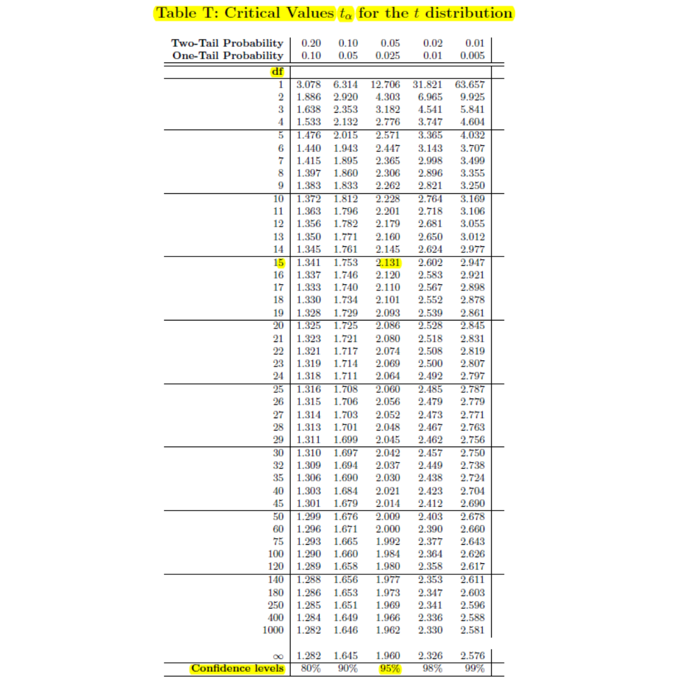
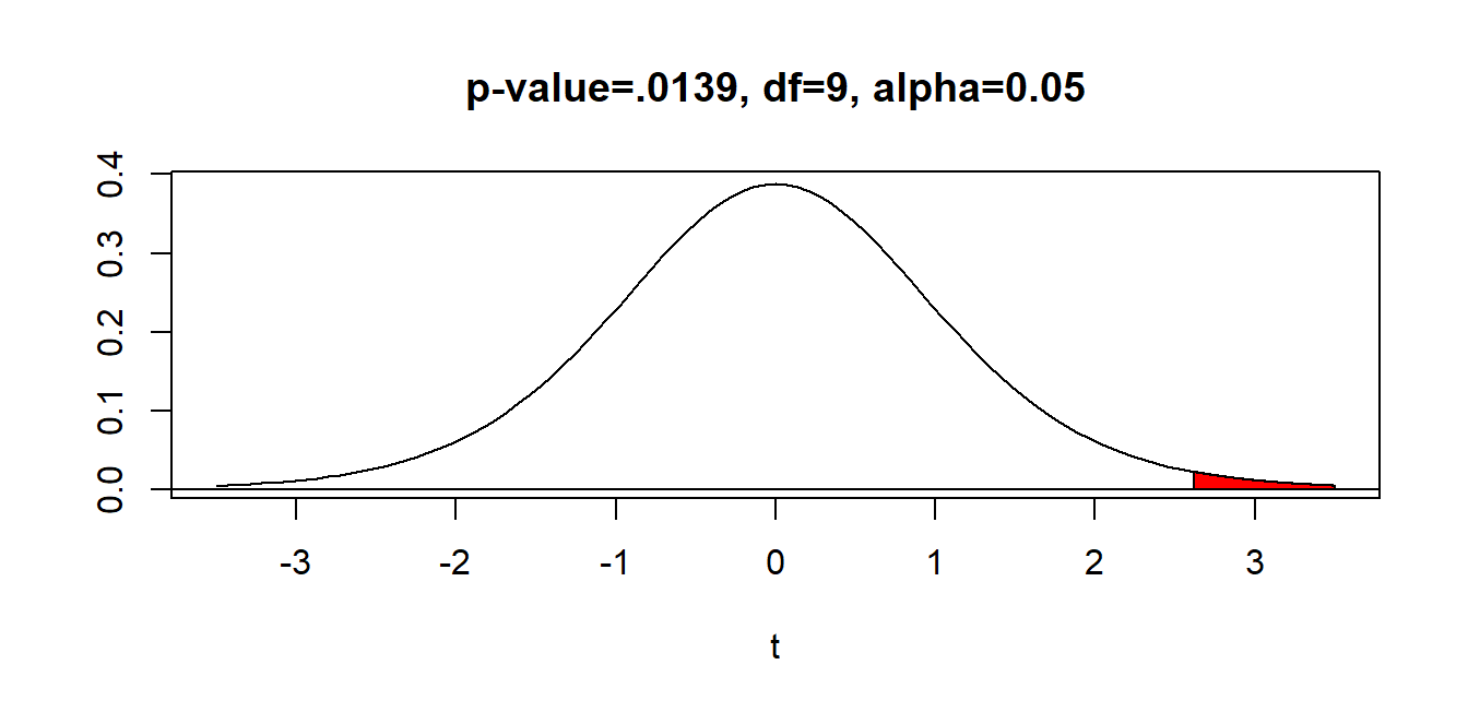
The \(p\)-value is \(P(t>2.62)\). With \(df=9\), notice our test statistic is between the critical values \(t^*=2.262\) and \(t^*=2.821\), which correspond to one-tail probabilities of \(0.025\) and \(0.01\), respectively. This means that \[0.01 < p-value < 0.025\]
Below is a picture showing the \(p\)-value, which can be computed with software to be \(p=0.0139\), which as promised is more than \(\alpha=0.01\) and less than \(\alpha=0.025\).
Since we are using \(\alpha=0.05\) and \(p < \alpha\), we REJECT the null hypothesis.
Step Six: Conclusion
The mean difference in reaction time decrease significantly after the subject drank alcohol.
Below is what statistical output from the software package R would look like for this problem. I also included output for the Wilcoxon Signed Rank test (even though we will not cover the formula for this test). The software includes a one-sided confidence interval that I’ll ignore.
##
##  Paired t-test
##
## data:  Before and After
## t = -2.62, df = 9, p-value = 0.01391
## alternative hypothesis: true mean difference is less than 0
## 95 percent confidence interval:
##        -Inf -0.0270305
## sample estimates:
## mean difference
##           -0.09
##
## Wilcoxon signed rank test with continuity correction
##
## data: Before and After
## V = 4, p-value = 0.01648
## alternative hypothesis: true location shift is less than 021.3 Confidence Interval
We could, of course, compute a confidence interval for the difference. Just like the hypothesis test for paired samples is just the one-sample \(t\)-test, we will just compute the one-sample \(t\)-interval.
One complication is that it is very common for paired samples \(t\)-tests to be one-sided, since we generally have a particular direction we expect the effect to be in. It is possible to compute a one-sided confidence interval (it appears in the computer output above), but I’m going to not present that formula and instead will just review confidence interval for a mean. Let’s do a 90% confidence interval.
\[\bar{d} \pm t^* \times \frac{s_d}{\sqrt{n}}\]
We have \(n=10\), so \(df=9\) and the critical value for 99% confidence is \(t^* = 1.833\).
\[0.09 \pm 1.833 \times \frac{0.1086}{\sqrt{10}}\]
\[0.09 \pm 1.833 \times 0.0343\]
\[0.09 \pm 0.063\]
\[(0.027,0.153)\]
21.4 Paired Samples \(t\)-test and CI with Technology
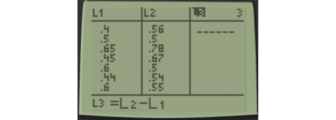
This test can be done with technology. I’ll demonstrate by first entering the \(X\) variable Before into List L1 and the \(Y\) variable After into List L2. It is critically important to keep the pairs on the same row, since we’ll be taking the difference. To not do so would be like if I entered your exam score into the wrong place in a spreadsheet, so someone else got your “A” and you got their “D”.
We then compute our difference \(D\) by taking After-Before or L3=L2-L1. I chose to subtract in that order since I expect the reaction time after drinking to be higher than before drinking, but you could do it the other way (Before-After).
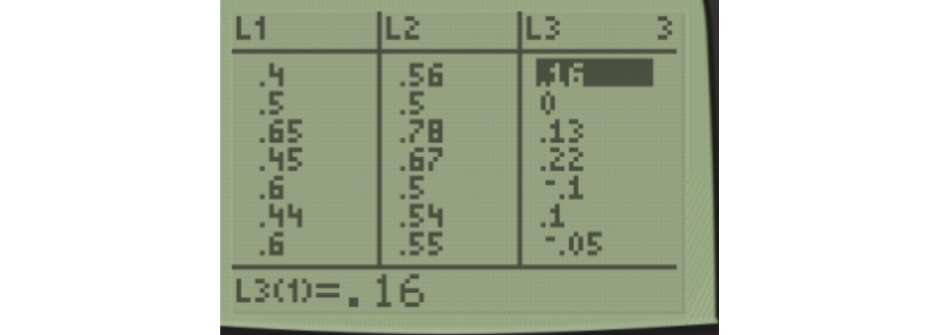
Once you hit ENTER and get values in List L3, then the paired samples \(t\)-test or confidence interval will just be doing the one-sample test or CI on the differences, as we did before.
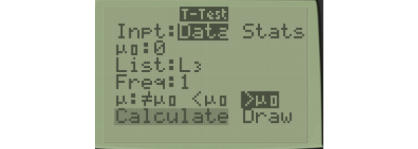
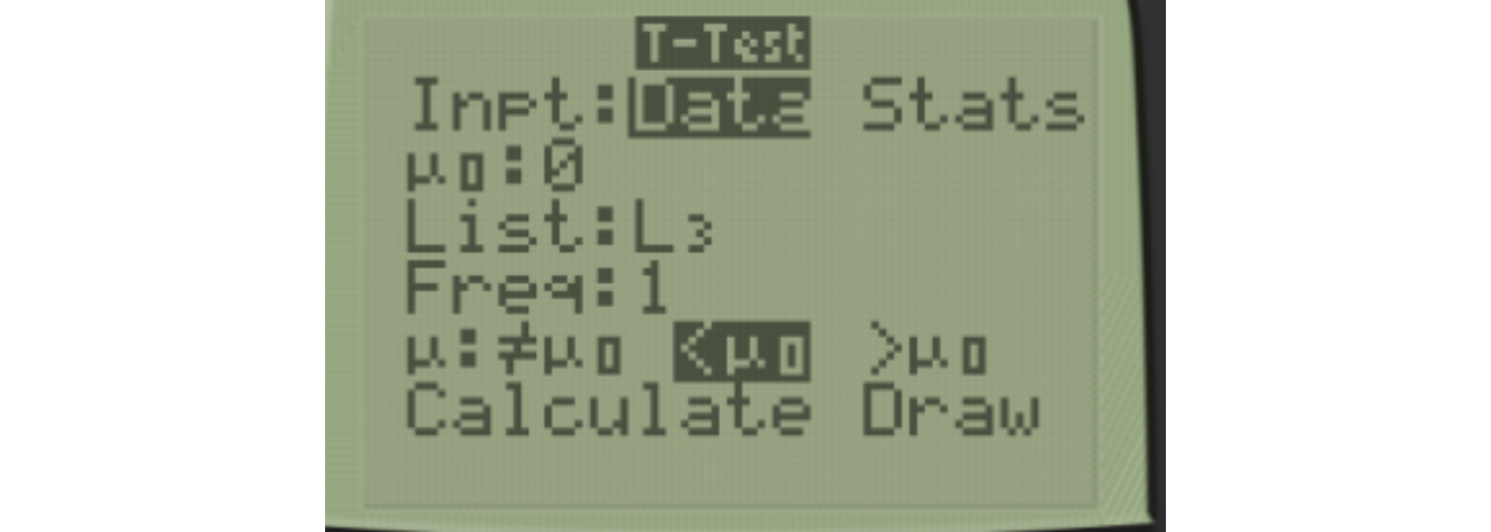
USe 2:TTest for the paired samples t-test. Notice I use List L3 since that is where the differences are stored. I chose \(H_a: \mu_d > 0\) since I expect the differences to be greater than zero (i.e. longer reaction time after drinking).
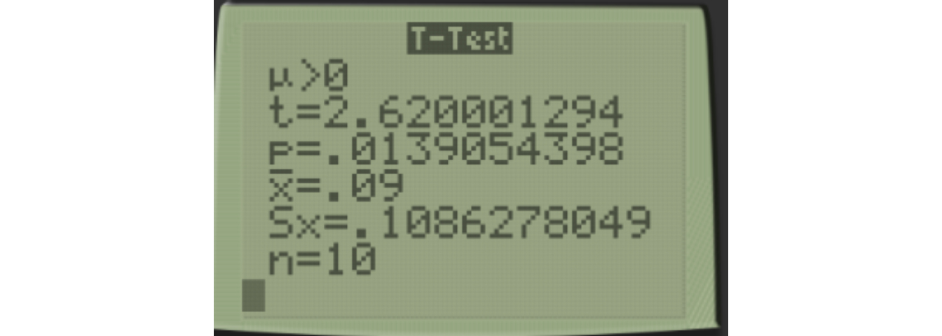
We get the same results as when we did it “by hand”. One thing to be careful about is picking the wrong direction, as that’s an easy mistake to make. A clue that you’ve picked the wrong direction is if your \(p\)-value is close to 1, as it will rarely be close to 1 for a one-sided test. Here I demonstrate making that mistake, notice I choose < by mistake.
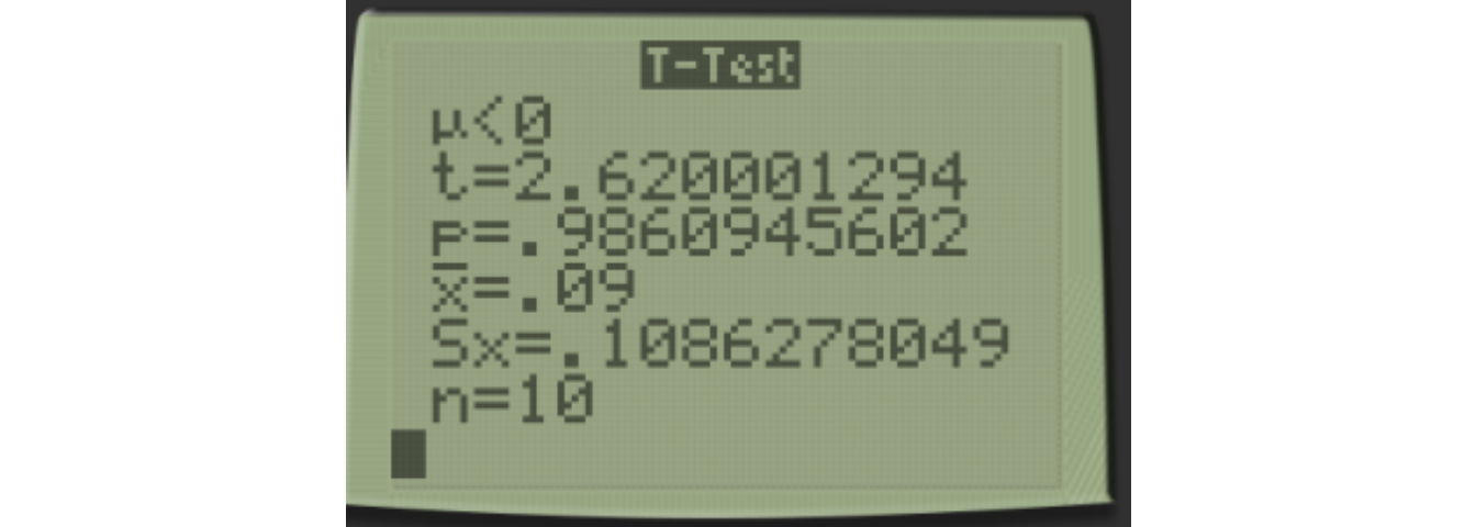
You can see the test statistic \(t\) is the same, \(t=2.620\), but the \(p\)-value is wrong and would lead you to the incorrect conclusion of failing to reject the null hypothesis if you didn’t realize your mistake.
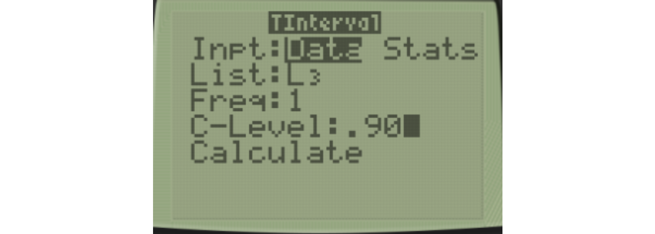
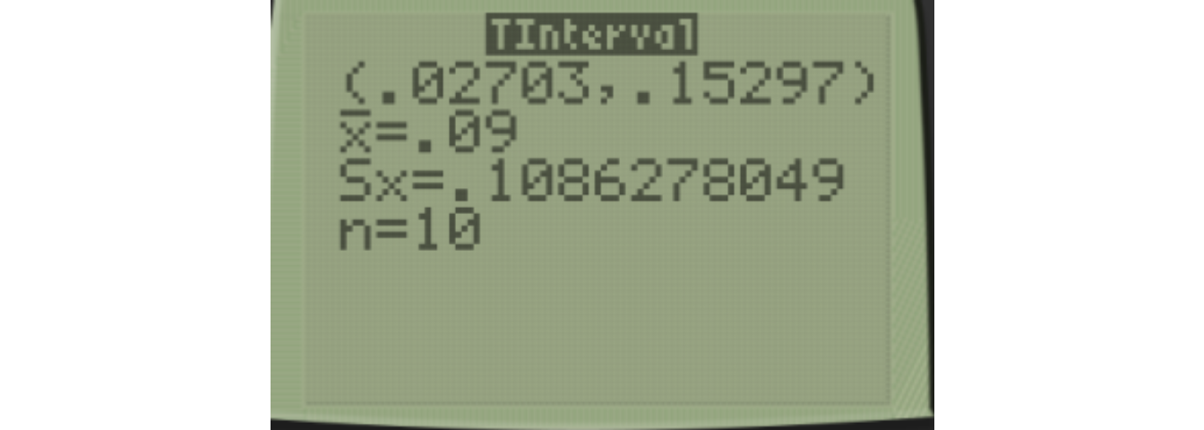
Finally, you can use 8:TInterval to get a confidence interval of the differences. I’ll do a 90% confidence interval as before, changing C-Level=.90.