Chapter 3 Relationships Between Categorical Variables
3.1 Contingency Tables
A contingency table or cross-tabulation (shortened to cross-tab) is a frequency distribution table that displays information about two variables simultaneously. Usually these variables are categorical factors but can be numerical variables that have been grouped together. For example, we might have one variable represent the sex of a customer in the store and the second variable be age, where age groups such as 18-29, 30-44, 45-64, 65+ are used.
Our hypothetical example looks at the ice cream preferences of a sample of people from two different states. I constructed a stacked bar chart to try to show the differences in ice cream preference between the states. I think you can see that blue portion (for Dippin’ Dots) is bigger in Kentucky than Vermont, and the red portion (for Ben and Jerry’s) is larger for Vermont than Kentucky.
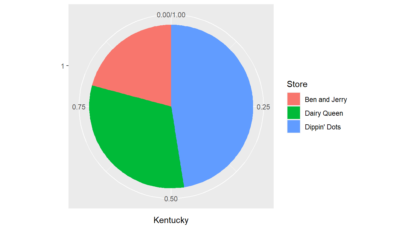
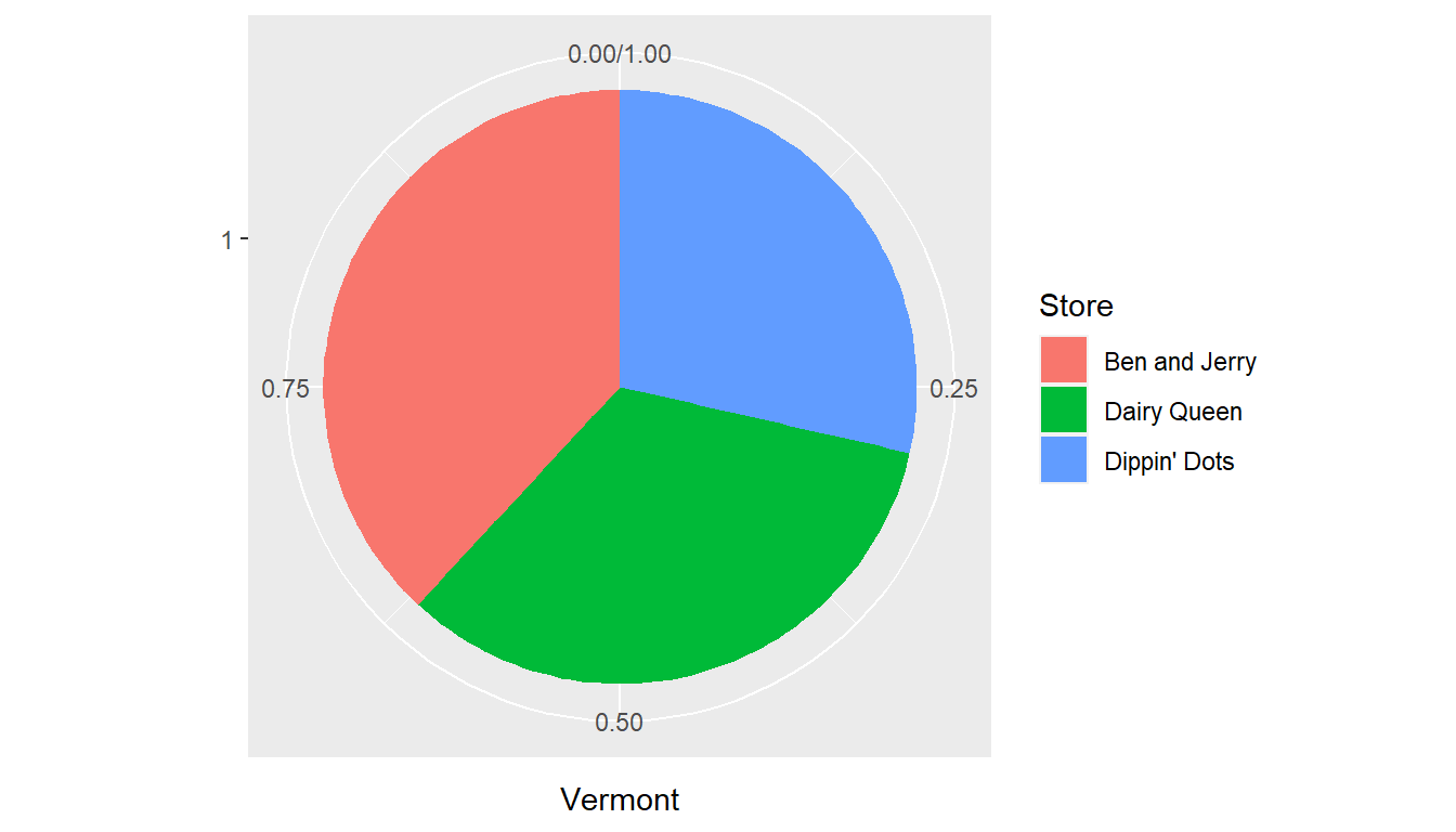
I also included pie charts for both states, although I think it is an inferior choice than the stacked bar charts.
##          Ben and Jerry Dairy Queen Dippin' Dots
## Kentucky            25          38           57
## Vermont             48          42           36
## # A tibble: 6 × 4
## # Groups: State [2]
## State Store Freq Prop
## <chr> <chr> <dbl> <dbl>
## 1 Kentucky Ben and Jerry 25 0.208
## 2 Vermont Ben and Jerry 48 0.381
## 3 Kentucky Dairy Queen 38 0.317
## 4 Vermont Dairy Queen 42 0.333
## 5 Kentucky Dippin' Dots 57 0.475
## 6 Vermont Dippin' Dots 36 0.286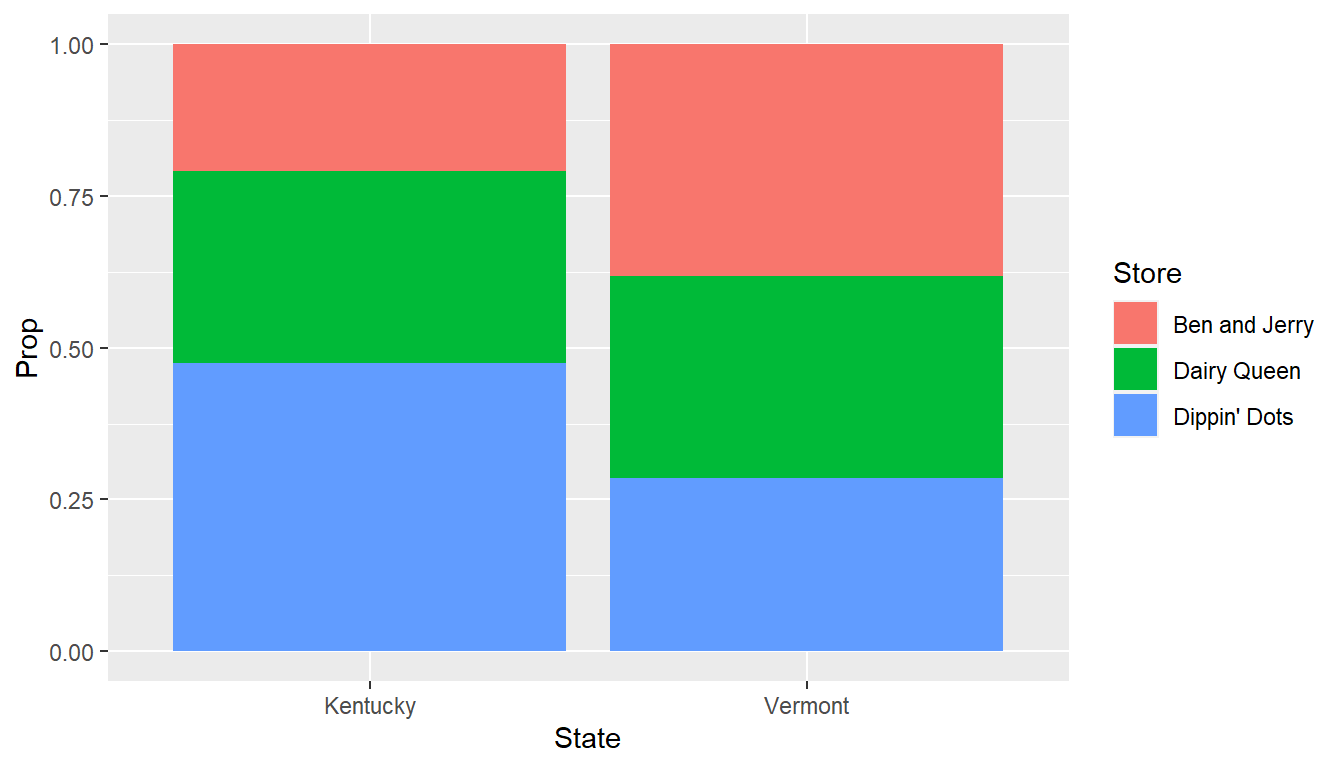
We can get marginal totals and percentages for both the rows (state) and columns (ice cream). We can also get conditional percentages for ice cream preference based on state; if these sets of percentages are the same for the two states, then we would say that they are indepedent (they aren’t here).
Here’s an example regarding the gender of STA 135 students from a previous semester and whether or not Los Portales was your favorite (number one choice) of the three restaurants or not, given as TRUE if it was your favorite and FALSE if not.
##
##          FALSE TRUE
##   Female    19   17
##   Male      13   10
This table is much closer to being statistically independent than the ice cream table.
3.2 Marginal Distributions
Marginal distributions is just another term for finding the distribution for a single variable at a time. Let’s take the contingency table for whether or not Los Portales was a student’s favorite restaurant by the student’s reported gender.
Let’s look at the row totals and the marginal distribution for gender (the row variable) first. There are \(19+17=36\) females and \(13+10=23\) males in the sample, with a total of \(n=59\) students. The marginal distributions is:
\[Female: \frac{36}{59}=0.610=61\%\]
\[Male: \frac{23}{59}=0.390=39\%\]
Do the same with the columns to get the marginal distribution based on Los Portales being your favorite restaurant in town. \(19+32=32\) students said it was not their favorite (FALSE), while \(17+10=27\) said that it was their favorite (TRUE).
\[\text{Not favorite (FALSE):} \frac{32}{59}=54.2\%\]
\[\text{Favorite (TRUE):} \frac{27}{59}=45.8\%\]
3.3 Conditional Distributions
A conditional distribution looks at the percentages for a variable GIVEN that the other variable takes on a specific value. In political polling, it is very common to look at conditional distributions to see who is the favorite candidate based on a variable such as gender, race, region of country, etc. It is often of interest to know, for example, if one candidate is more or less popular when comparing men versus women, whites versus people of color, etc.
Here, we’ll see if there is a difference between female and male students in whether they ranked Los Portales as their favorite restaurant.
\[Favorite,Female: \frac{17}{36}=47.2\%\]
\[Favorite,Male: \frac{10}{23}=43.5\%\]
If the two variables are statisically independent, these two percentages would be exactly the same. They aren’t exactly equal, but are pretty close, so it doesn’t seem like there’s a meaningful differece between female and male students in terms of liking Los Portales.
3.4 Polling Example
Here’s an example of a recent poll based on President Trump’s approval rating as the impeachment trial in the Senate is beginning. Later this semester, we’ll study how to compute and interpret the margin of error and how to collect such a random sample.
This poll was collected between January 2nd and January 15th, 2020 and consisted of a random sample of \(n=1014\) adults across the U.S.A. As you see at the top of the article, the overall approval rating for Trump was 44%, and a time series plot showings this trend for this question over the past year.
https://news.gallup.com/poll/283364/senate-trial-begins-approve-trump.aspx
If you click on the link for View complete question response and trends you will see this broken down by various demographic variables. It will probably not come as a surprise to you that the conditional distributions for variables such as gender, race, or political preference are quite different, as these variables are NOT independent. Certain portions of the population support President Trump by a much greater percentage than 44%, and others much less than 44%.
For instance, the presidential approval rate is 55% for males and 34% for females. Looking at race, it is 56% for whites and 21% for non-whites. On political ideology, it is 71% for conservatives, 35% for moderates, and 7% for liberals.
3.5 Simpson’s Paradox
Video: https://youtu.be/ebEkn-BiW5k (treating cats vs humans)
Florida death penalty example A well-known statistician (Alan Agresti) worked with sociologists at the University of Florida in the late 1970s and early 1980s, as they were studying data involving what factors led to people convicted of first-degree murder being sentenced to death or not. One’s initial guess might be to guess that black defendants will be more likely to receive the death penalty than white defendants, given the location and time period.
##          Penalty
## Defendant  No Yes
##     Black 149  17
##     White 141  19
I’ll turn the contingency table into some conditional percentages and a graph. You can see that the percentage of murderers receiving the death penalty is virtually the same between the two races; in fact, it’s actually slightly higher for the white murderers.
## # A tibble: 4 × 5
## # Groups:   Defendant [2]
##   rowname Defendant Penalty  Freq  Prop
##   <chr>   <fct>     <fct>   <int> <dbl>
## 1 1       Black     No        149 0.898
## 2 2       White     No        141 0.881
## 3 3       Black     Yes        17 0.102
## 4 4       White     Yes        19 0.119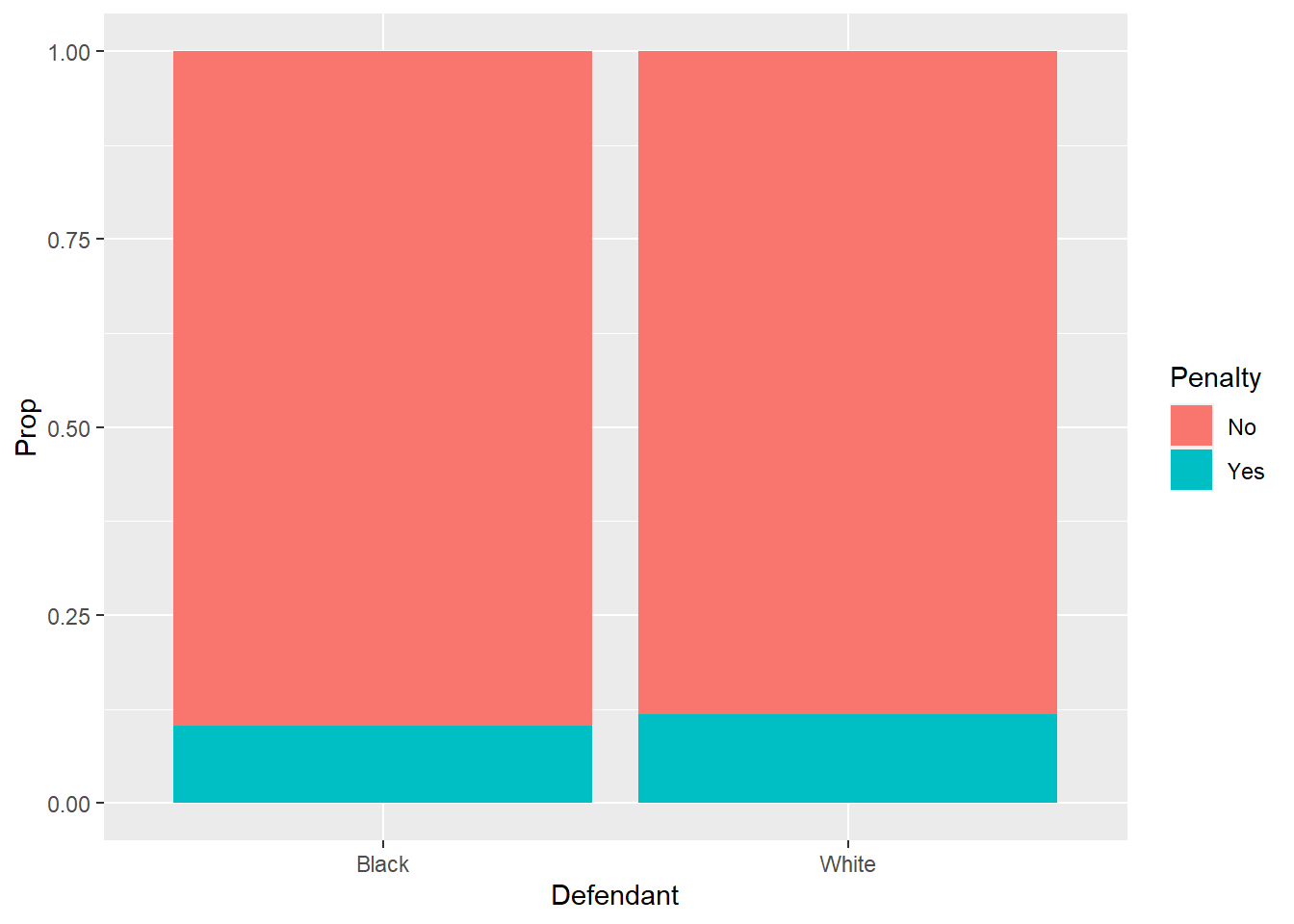
But not everything is neatly described by two and only two variables. Here, the race of the victim (the person that was murdered) was also studied. Maybe the victim’s standing in society played a role in the fate of the convicted criminal?
It’s a bit more complicated, but we can study a three-way contingency table. We end up seeing that the black murderer ends up being more likely to receive the death penalty than the white murderer when we break it down on the victim’s race. The criminal is more likely to receive the death penalty when their victim is white. Since most murders involve both the murderer and victim being the same race (and usually know each other), this explains why the percentage was higher for white criminals when the victim’s race was not considered (i.e. an explanation for the paradox).
## , , Victim = Black Victim
##
##          Penalty
## Defendant  No Yes
##     Black  97   6
##     White   9   0
##
## , , Victim = White Victim
##
##          Penalty
## Defendant  No Yes
##     Black  52  11
##     White 132  19
## # A tibble: 8 × 6
## # Groups: Defendant, Victim [4]
## rowname Defendant Penalty Victim Freq Prop
## <chr> <fct> <fct> <fct> <int> <dbl>
## 1 1 Black No Black Victim 97 0.942
## 2 2 White No Black Victim 9 1
## 3 3 Black Yes Black Victim 6 0.0583
## 4 4 White Yes Black Victim 0 0
## 5 5 Black No White Victim 52 0.825
## 6 6 White No White Victim 132 0.874
## 7 7 Black Yes White Victim 11 0.175
## 8 8 White Yes White Victim 19 0.126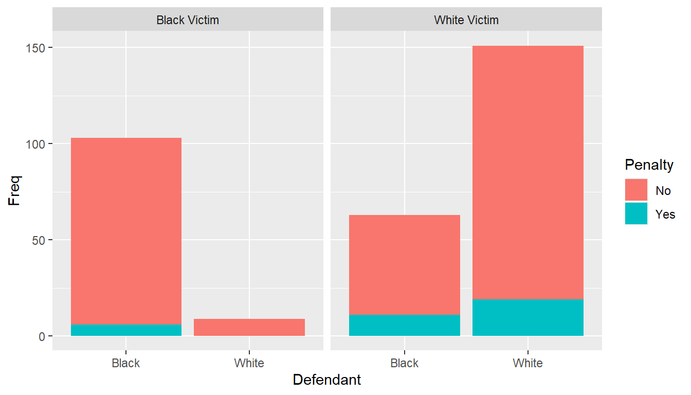
Radelet, M. (1981), “Racial Characteristics and Imposition of the Death Penalty,” American Sociological Review, 46, 918-927.
Professor Agresti used this example in a textbook he wrote and many others have used it since
Incidentally, Michael Radelet’s article concludes with this paragraph:
“In conclusion, relative equality in the imposition of the death penalty appears mythical as long as prosecutors are more likely to obtain first degree murder indictments for those accused of murdering white strangers than for those accused of murdering black strangers. Racial differences in the processing of those indicted for nonprimary homicides in Florida appears to place a lower value on the lives of blacks than on the lives of whites.”
Radelet is now at the University of Colorado and has been anti-death penalty since the 1970s. Based on a Google search, I found this article about him on the website of an organization that wants to abolish the death penalty.
https://deathpenalty.org/blog/the-focus/voices-michael-radelet/
Here’s another website with pros and cons.
https://deathpenalty.procon.org/view.answers.php?questionID=001324
This is an example of Simpson’s Paradox. Simpson (1951) demonstrated that a statistical relationship observed within a population — i.e., a group of individuals — could be reversed within all subgroups that make up that population. This phenomenon, where \(X\) seems to relate to \(Y\) in a certain way, but flips direction when the population is split for a third varaible \(W\), has since been referred to as Simpson’s paradox. Others names, according to Wikipedia, include the Simpson-Yule effect, reversal paradox or amalgamation paradox.
In the death penalty example, \(X\) is the race of the murderer and \(Y\) is the sentence they received, where the lurking variable \(W\) is the race of the victim.
Sources: https://paulvanderlaken.com/2017/09/27/simpsons-paradox-two-hr-examples-with-r-code/
3.6 Another Simpson’s Paradox example
Example 3.8 on page 80-81 of the textbook is another famous example of Simpson’s paradox, based on whether or not admission to graduate school at the University of California-Berkeley showed gender-based discrimination or not. As in the Florida death penalty case, the story the data tells is different when all three important variables (gender, whether the student was admitted or not, what department the student applied to) is different than the story if one of the variables (which department) is omitted.
Here’s the video for that example: https://youtu.be/E_ME4P9fQbo