Chapter 13 Probability Rules and Bayes Theorem
13.1 General Addition Rule
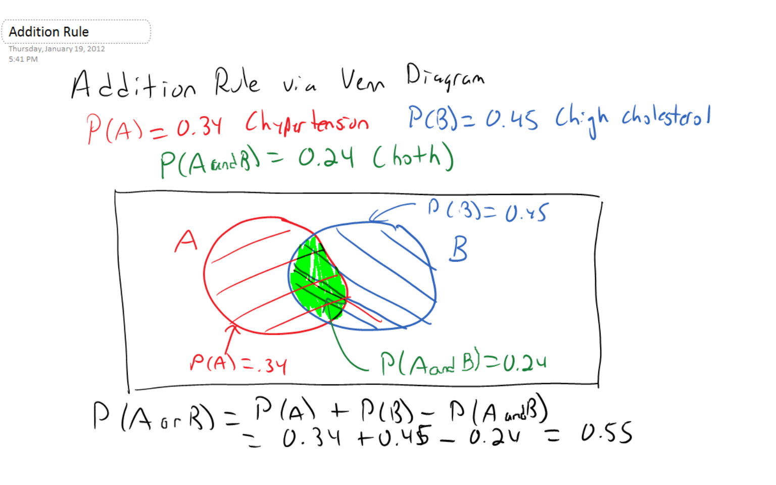
Suppose event \(A\) is the event that a middle-aged person has hypertension and event \(B\) is the event that they have high cholesterol. Obviously a person could have both of these conditions; in other words, events \(A\) and \(B\) are NOT mutually exclusive.
Suppose we know that \(P(A)=0.34\), \(P(B)=0.45\), and \(P(A \: and \: B)=0.24\), where \(A \: and \: B\), sometimes written \(A \cap B\) is the intersection, or the probability of event A AND event B (i.e. having both hypertension and high cholesterol).
13.2 Addition Rule
We want to know \(P(A \: or \: B)\), sometimes written \(A \cup B\), the intersection, or the probability of event A OR event B. The addition rule states:
\[P(A \: or \: B)=P(A)+P(B)-P(A \: and \: B)\]
In our medical example, \[P(A \: or \: B)=0.34+0.45-0.24=0.55\]
We subtract the probability of the intersection to correct for the fact that we would ‘double count’ those individuals with both hypertension and high cholesterol if we did not.
If events \(A\) and \(B\) are mutually exclusive, then \(P(A \: and \: B)=0\).
13.3 Complement Rule
The complement of an event is the probability of all outcomes that are NOT in that event. For example, if \(A\) is the probability of hypertension, where \(P(A)=0.34\), then the complement rule is: \[P(A^c)=1-P(A)\]
In our example, \(P(A^c)=1-0.34=0.66\). This may seen very simple and obvious, but the complement rule can often save a lot of work, in situations where finding the probability of an event is difficult or impossible but the probability of its complement is relatively easy to find.
13.4 DeMorgan’s Laws
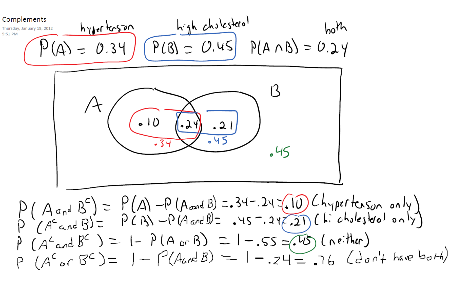
\(P(A \: and \: B^c)=P(A)-P(A \: and \: B)=0.34=0.24=0.10\) This is the probability of event A only (hypertension and NOT high cholesterol)
\(P(A^c \: and \: B)=P(B)-P(A \: and \: B)=0.45-0.24=0.21\) This is the probability of event B only (high cholesterol and NOT hypertension)
\(P(A^c \: and \: B^c)=1-P(A \: or \: B)=1-0.55=0-.45\). This is the probability of having neither hypertension nor high cholesterol.
\(P(A^c \: or \: B^c)=1-P(A \: and \: B)=1-0.25=0.76\). This is the probability of not having both conditions.
The last two formulas are referred to as De Morgan’s Laws.
13.5 Conditional Probability
Often, knowing that one event has occurred changes the probability of another event. For example, a certain percentage of the population is known to be positive for the HIV virus. If we gain further knowledge on an individual, that could make it more or less likely they are HIV positive. Someone who is a known heroin addict and engages in risky sexual behaviors would have a greater chance, while someone who is a virgin would have a much lower probability.
We use the notation \(P(A|B)\) to denote the conditional probability of \(A\), if \(B\) has occurred. The following formula formalizes this concept: \[P(A|B)=\frac{P(A \: and \: B)}{P(B)}\]
In the hypertension/high cholesterol example, we would have:
\[P(A|B)=\frac{0.24}{0.45}=\frac{8}{15}=0.5\bar{3}\]
Notice that one is more likely to have hypertension IF they also have high cholesterol. This probability seems to make sense, as these health problems are related and are not independent of each other.
In our homework example, we might find that children who like one kind of fruits (bananas) are also more likely to like another kind of fruit (apples). In politics, we might find that one’s sex is not independent of political preference. Female voters are often more likely to vote for Democrats than males, and males are more likely to vote for Republicans than females.
13.6 Independent and Dependent Events (Dice Rolling)
As we saw on the previous slide, events are often related, or dependent.
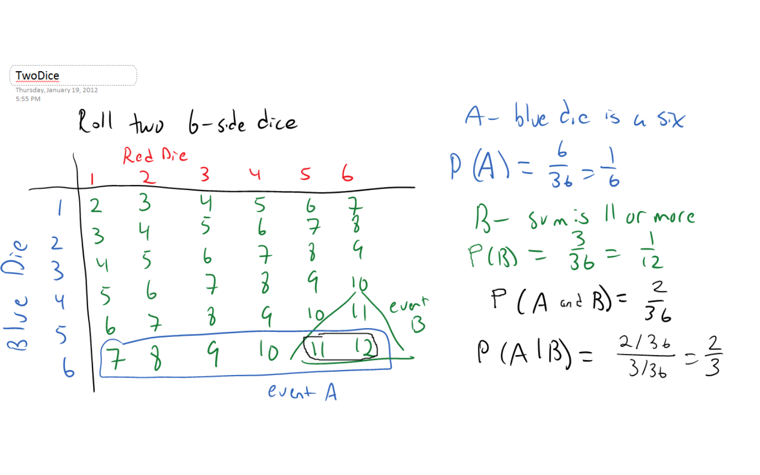
Consider the following situation: two 6-sided dice, one that is blue and one that is red, are rolled. Let \(X\) represent the sum of the two dice. There are \(6 \times 6=36\) possible dice rolls. The possible values of \(X\) are \(2,3,4,\cdots,10,11,12\).
Let event \(A\) be the event that the blue die is a `6’ and event \(B\) be the event that the two dice sum to 11 or more (i.e. \(X=11\) or \(12\)). The probabilities of these two events separately are \(P(A)=1/6\) and \(P(B)=3/36=1/12\). However, \(P(A \: and \: B)=2/36\) and \[P(A|B)=\frac{2/36}{3/36}=\frac{2}{3}\]
Since \(P(A) \neq P(A|B)\), these events are NOT independent of one another.
Now consider event \(A\), the event that the blue die is a `6’ and event \(B\), the event that the red die is even. The two dice have no impact on the result of the other dice.
Notice \(P(A)=1/6\), \(P(B)=3/6\) and \(P(A \: and \: B)=3/36\). So \[P(A|B)=\frac{3/36}{3/6}=\frac{6}{36}=\frac{1}{6}=P(A)\]
Since \(P(A)=P(A|B)\), the two events are mathematically independent.
13.7 Multiplication Rule
The multiplication rule is used to find the probability of an intersection \(P(A \cap B)\), or \(A\) AND \(B\).
\[P(A \: and \: B)=P(A|B)\times P(B)\]
When the events are independent, then \(P(A|B)=P(A)\) and the rule simplifies to \[P(A \: and \: B)=P(A) \times P(B)\]
The tree diagram on the next slide looks at the probability of being dealt a pair of aces in holdem poker (dependent events) and the probability of flipping a coin twice and getting two heads (independent events).
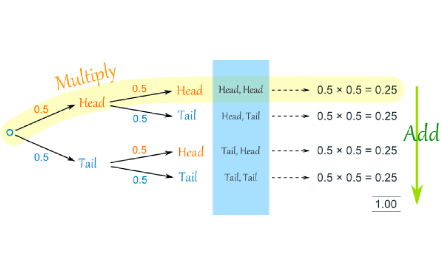
13.8 Coin Flipping (independent)
Let \(H_1\) represent flipping a coin and getting heads. Let \(H_2\) represent flipping a second coin and getting heads. It is known that \(P(H_1)=\frac{1}{2}\) and that \(P(H_2)=\frac{1}{2}\).
How can we find the probability that both events occur, i.e. \(P(H_1 \quad and \quad H_2)\)? How about exactly one of the two events? Neither of the two events?
We’ll use the multiplication rule and construct a tree diagram.
The probability of both events is: \[P(H_1 \quad and \quad H_2)=P(H_1)\times P(H_2)=\frac{1}{2} \times \frac{1}{2}=\frac{1}{4}\].
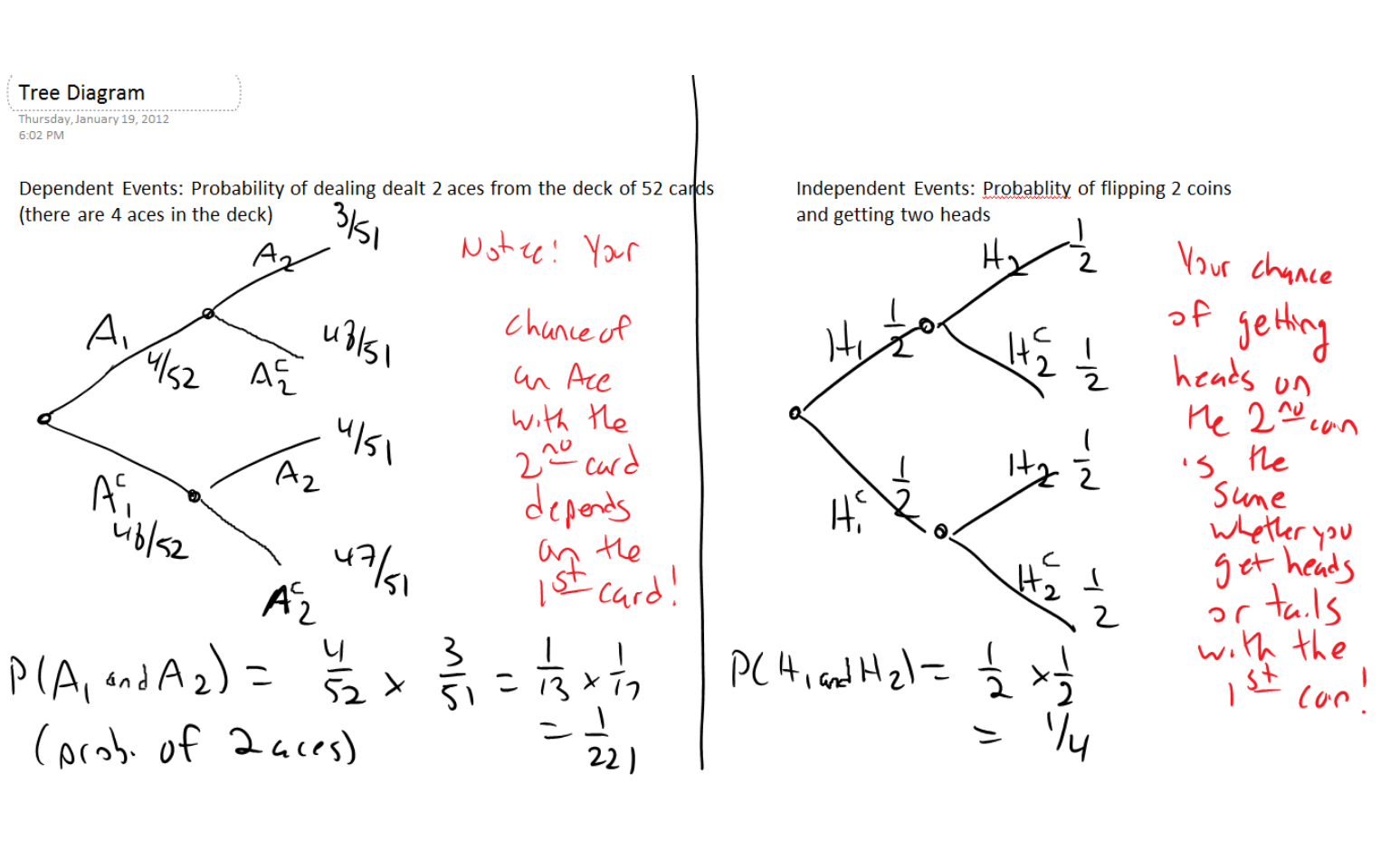
13.9 Texas Holdem (dependent events)
Now we are going to play Texas holdem poker. In this game, you begin by being dealt 2 cards without replacement from the standard 52-card deck. Let \(A_1\) be the event that your first card is an Ace and \(A_2\) the event the second card is an ace.

How can we find the probability of getting two aces (what poker players call “pocket aces” or “pocket rockets”)? How about the probability of a hand with exactly one ace? A hand with no aces?
This will be similar to the coin/dice problem, and we’ll use the multiplication rule and a tree diagram again, but with an important difference.
Here, \(P(A_1)=\frac{4}{52}=\frac{1}{13}\) since the standard 52-card deck contains 4 aces.
However, \(P(A_2)\) depends on what the first card was. In the previous problem, your chance of getting doubles when you roll the two dice is unrelated to whether you got heads or tails when you flipped the coin. But if your first card is an ace, there are only 3 aces left and \(P(A_2|A_1)=\frac{3}{51}=\frac{1}{17}\). However, if the first card is not an ace, then there are still 4 aces left: \(P(A_2|A_1^c)=\frac{4}{51}\)
The probability of both events (getting 2 aces) is: \[P(A_1 \: and \: A_2)=P(A_1) \times P(A_2|A_1)=\frac{4}{52} \times \frac{3}{51}=\frac{1}{13} \times \frac{1}{17} = \frac{1}{221}\]
13.11 Contingency Table
A common way to be presented quantitative data is in a two-way contingency table, where the rows of the table classify the subjects on one variable and the columns on a second variable.
For our example, we will have a \(2 \times 3\) contingency table; the 2 rows will represent boys and girls and the 3 columns will represent three different flavors of ice cream that might be their favorite.
##       Chocolate Vanilla Strawberry
## Boys         75      75         50
## Girls       150     100         50
The marginal row totals are 200 and 300 (there are 200 boys and 300 girls, for a total of 500 children). The marginal column totals are 225, 175, and 100 (225 like chocolate, 175 vanilla, 100 strawberry).
\(P(Boy)=\frac{200}{500}=\frac{2}{5}=0.40\); 40% of the sample are boys
\(P(Girl)=\frac{300}{500}=\frac{3}{5}=0.60\); 60% of the sample are girls
\(P(Chocolate)=\frac{225}{500}=0.45\); 45% of the children prefer chocolate ice cream
\(P(Boy \: and \: Chocolate)=\frac{75}{500}=0.15\) 15% of the children are boys that prefer chocolate ice cream
\(P(Boy \: or \: Chocolate)=\frac{200}{500}+\frac{225}{500}-\frac{75}{500}=\frac{350}{500}=0.70\); notice we subtract the intersection to avoid double-counting the boys that like chocolate; this counts all boys and also the girls that like chocolate
\(P(Chocolate|Boy)=\frac{75/500}{200/500}=\frac{75}{200}=0.375\); 37.5% of the boys like chocolate the most
\(P(Chocolate|Girl)=\frac{150/500}{300/500}=\frac{150}{300}=0.5\); 50% of the girls like chocolate the most
Girls are more likely and boys less likely to prefer chocolate; the events are NOT independent.
13.12 Bayes’ Theorem
This famous theorem, due to the 18th century Scottish minister Reverend Thomas Bayes, is used to solve a particular type of ‘inverse probability’ problems.
The usual way of stating Bayes’ Theorem, when there are only two possible values, or states, for event \(B\), is: \[P(B|A)=\frac{P(A|B) \times P(B)}{P(A|B) \times P(B) + P(A|B^c) \times P(B^c)}\]
where \(P(B)\) is called the probability of the event and the final answer, \(P(B|A)\) is the or revised probability based on information from event \(A\).
Bayes’ Theorem is often used in medicine to compute the probability of having a disease GIVEN a positive result on a diagnostic test. We will replace \(A\) and \(A^c\) in the previous formula with \(T^+\) and \(T^-\) (reprenting a positive and negative test result). We will also replace \(B\) with \(D^+\), representing having the disease. \(B^c\) is replaced by \(D^-\), not having the disease.
\[P(D^+|T^+)=\frac{P(T^+|D^+) \times P(D^+)}{P(T^+|D^+) \times P(D^+) + P(T^+|D^-) \times P(D^-)}\]
Suppose the prevalence (i.e. prior probability) of having Martian flu is \(P(D^+)=0.01\). Therefore \(P(D^-)=1-0.01=0.99\), which is not having the disease.
The sensitivity of the test is 95%, so \(P(T^+|D^+)=0.95\) (‘true positive’)
\(P(T^-|D^+)=1-0.95=0.05\) (‘false negative’-a bad mistake to make!)
The specificity of the test is 98%, so \(P(T^-|D^-)=0.98\) (‘true negative’)
\(P(T^+|D^-)=1-0.98=0.02\) (‘false positive’)
Solving with a formula:
\[P(D^+|T^+)=\frac{P(T^+|D^+) \times P(D^+)}{Pr(T^+|D^+) \times P(D^+) + P(T^+|D^-) \times P(D^-)}\]
\[P(D^+|T^+)=\frac{0.95 \times 0.01}{0.95 \times 0.01 + 0.02 \times 0.99}\]
\[P(D^+|T^+)=\frac{0.0095}{0.0095+0.0198}\]
\[P(D^+|T^+)=\frac{0.0095}{0.0293}\]
\[P(D^+|T^+)=0.3242\]
Solving with a tree diagram:
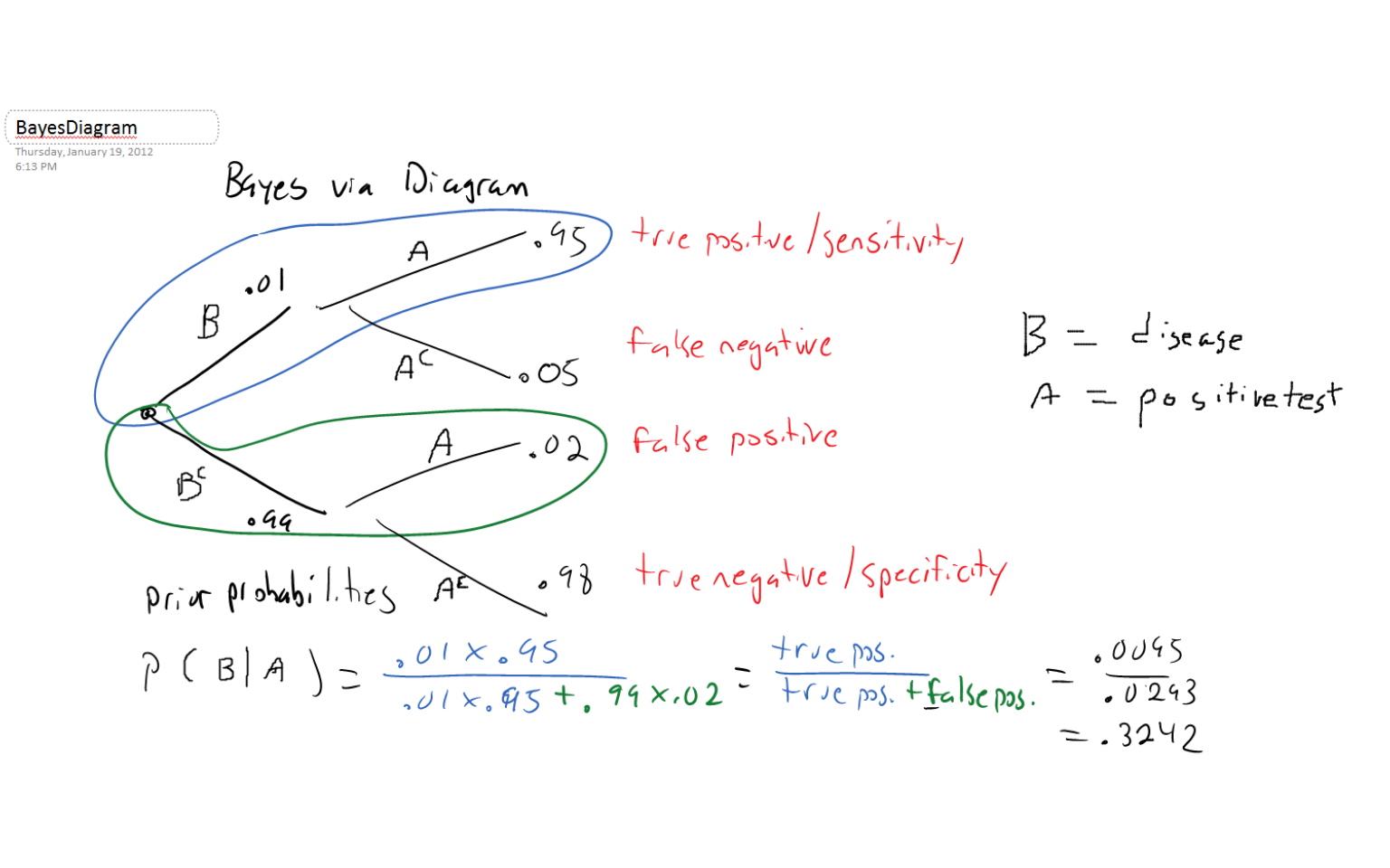
Notice that \(P(D^+|T^+)\), the probability of having Martian flu if you had a positive test, is only 32.42%. This probability is so low because there are actually more ‘false positives’ than ‘true positives’ in the population.
This is often the case for rare diseases (i.e. low prevalence) unless sensitivty and specificity are incredibly close to 1.
A very nice online tool for seeing this tree diagram is here:
http://www.harrysurden.com/projects/visual/Probability_Tree_D3/Probability_Tree_D3.html
While this will be the extend of our foray into Bayesian statistics, there is a large body of work in applied statistics that build upon the old reverend’s theorem for reversing probabilities!
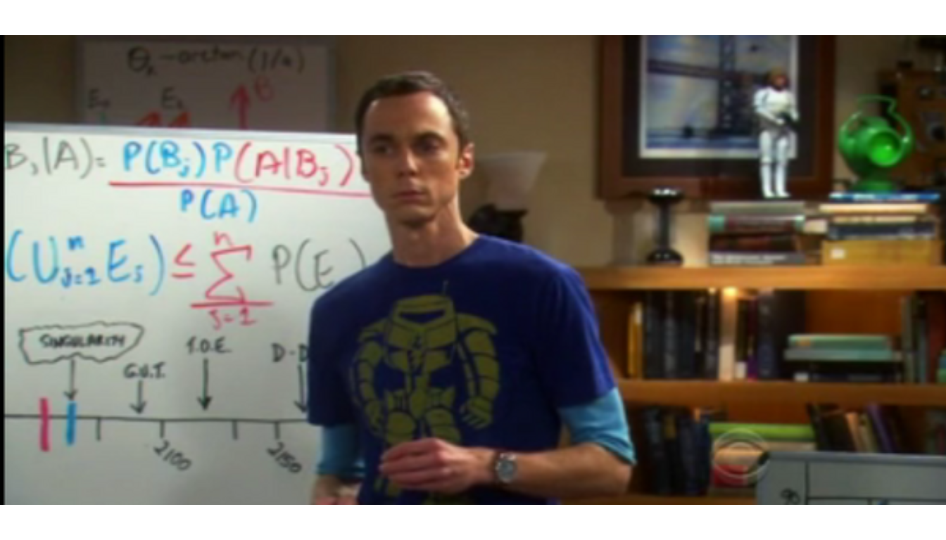
Sheldon Cooper from the sitcom The Big Bang Theory is using Bayes’ Theorem (with slightly different notation), along with a result called Boole’s Inequality that we won’t cover. I saw more Bayesian statistics on Sheldon’s whiteboard on a more recent episode, but I didn’t track down the screenshot.