Chapter 11 Experiments and Observational Studies

11.1 Association

Two variables are associated if values of one variable tend to be related to the values of the other variable. For example, I might notice that students who report studying for more hours per week also tend to be the students with the highest G.P.A.

The variables are causually associated if changing the value of one variable influences the value of the other variable.

This means if we manipulate one variable, we can change the other variable. For example, a farmer might notice that if they increase the amount of fertilizer used on a field, the yield of corn will increase. (Which is the explanatory variable and which is the response variable?)

Of course, this trend might not hold forever. If the farmer uses too much fertilizer, at some point it will actually cause the yield to decrease, as the farmer might actually kill the crop.

Just because two variables are associated doesn’t mean that there is a causal relationship. For example, suppose you own an ice cream store near the beach. You might notice that the months of the year that have the highest ice cream sales are also the months of the year with the highest number of shark attacks! This doesn’t mean eating ice cream before swimming will make sharks more likely to attack. Here, there is a confounding factor, or lurking variable that is associated with both the explanatory variable (shark attacks) and response variable (ice cream sales), in this case the time of year or the temperature. You will sell more ice cream in the summer, when more people go swimming, and thus there is a greater chance of a shark attack.

11.2 The Physicians’ Aspirin Study

In the 1980s, a study was designed to see if taking aspirin would be beneficial in reducing the chance of suffering a heart attack. A sample of approximately 22000 middle-aged male physicians was collected. Half were randomly assigned to take aspirin, and the other half a placebo, or inert substance that did not contain aspirin. Both the participants in the study and the doctors & nurses that they interacted with were unaware of whether they were in the treatment group (aspirin) or the control group (placebo).

After the data was collected and analyzed statistically, it was shown that the physicians in the treatment group were significantly less likely to have suffered a heart attack during the time period of the study than those in the control group. (consider Table 1.1 from the textbook)

Condition	Heart Attack	No Heart Attack	Attacks per 1000
Aspirin	104	10,933	9.42
Placebo	189	10,845	17.13

The rate of heart attacks in the aspirin group was \[\frac{9.42}{17.13}=0.55\] only 55% what was observed in the placebo group.

This study was the basis of the common recommendation of taking a low-dose aspirin tablet to reduce one’s chance of having a heart attack. You may have seen the commericials that some aspirin companies have on TV that advertise this fact and encourage viewers to see their doctor to see if they should go on an ‘aspirin regimen’.

A medical journal would include more sophisticated statistics like the risk ratio, odds ratio, confidence intervals with margins of error for these statistics, or the results of a statistical procedure such as the chi-square test. See vassarstats.net/odds2x2.html for an online calculator of these, if you like. Why might it be unlikely to include this information in an article meant for the general public?

This difference would have occured by chance only about 1 in 100,000 times (this is a statistic called the \(p\)-value which we cover later.)

More details of the study are found here: http://phs.bwh.harvard.edu/phs1.htm

11.3 Questions about the Aspirin Study

1. Do you think the sample used in this study was collected in an appropriate fashion?

2. If you were going to redo this study, would you change anything about how the sample was collected?

3. Do you have any other concerns about how the study was conducted?

11.4 Designed Experiments: Single Group Design

Let us reconsider the Physicians Aspirin Study example? How come the researchers didn’t select a single group design for this experiment.

In other words, how come the experiment wasn’t just: gather a large sample of subjects (in that experiment, middle-aged male physicians), give the subject the treatment (aspirin), and measure to see if the desired outcome (reduction in rate of heart attacks) occurs?

11.5 Designed Experiments: Single Group Design

The problem is that the effect of the independent variable (aspirin) on the dependent variable (rate of heart attacks) cannot be separated from other extraneous variable(s). These extraneous variable(s) may or may not even be known to the researchers and are called confounding variables.

The presence of confounding variables would make it impossible to attribute a reduction in heart attack rate to the aspirin. Maybe everyone in the study decided to exercise more or improve their eating habits.

11.6 Observational Study

In an observational study, no control is placed on the independent variables. Common examples of observational studies are sample surveys. Even though no control of the independent variables are used, this is often an appropriate design. For example, if I want to know the opinions of the American public on health insurance, I would not want to manipulate the subjects into answering a certain way.

In a planned experiment, the researcher do manipulate, or control, the values of independent variable(s). In the aspirin study, this was done by randomly assigning the subjects to receive either aspirin or a placebo. If there is a difference in the response between the two compariosn groups, we can attribute the difference to the treatment. In the aspirin study, there was a statisically significant decrease in rate of heart attacks when aspirin was taken.

11.7 Single Factor Design

Randomization is typically used in planned experiments to assign experimental units to different levels of an independent variable, or factor. This random selection used to be done with random number tables, but now is typically done via random number generators on computers.

Consider a single factor design. We are studying the effectiveness of a `patch’ to help people quit smoking. Suppose we have three levels of the factor: a patch with a high dose of the active agent, a patch with a low dose of the active agent, and a patch with no dose of the active agent, which serves as a placebo. If we had \(n=300\) subjects, we could randomly assign 100 to each level of the dose and determine what level of dose is most effective.

11.8 Types of Randomzied Experiments

– Randomized comparative experiment, we randomly assign cases to different treatment groups and then compare results on the response variable.

– Matched Pairs experiment, each case gets both treatments in random order and we look at individual differences in the response variable between the two treatments. Sometimes cases get “paired up”, such as pairing you with the person in the study most similar to you. Twins are ideal for this design, with one twin getting one treatment and the other the second treatment.

11.9 Factorial Design

Now consider a more complicated two factor design, where we want to study both the dose (high/low/placebo) and method of delivery (patch/gum). We have 3 levels of dose (what level of dose is best?) and 2 levels of method (is the patch better/worse than the gum?), so we have \(3 \times 2=6\) different treatments. With a smaple of \(n=300\), we would randomly assign 50 subjects to: patch-high, patch-low, patch-placebo, gum-high, gum-low, gum-placebo. We would determine what combination of dose and method is most effective.

We could have three or more factors as well in such a factorial design.

11.10 Randomized Block Design

The designs we have considered so far are completely randomized designs, where the randomization of subjects to groups happens without any restriction. In my smoking example, the researcher would have complete control over whether a subject received the patch or the gum and what level of dose they received.

Often there are extraneous variables, or factors, of interest that we cannot control via randomization. In the smoking example, we might want to compare heavy smokers (more than one pack/day) versus light smokers (less than one pack/day). It would not be appropriate (or possible) to randomly assign subjects to smoke a certain amount of cigarettes, so we would use the technique called blocking.

If I had 120 heavy smokers and 180 light smokers in my study, looking at a patch with either a high/low/no dose, I would use the level of smoking as a block, randomly assign 40 heavy smokers to each dosage group, and randomly assign 60 light smokers to each dosage group.

Variables such as sex, age, etc. which cannot be randomly controlled are commonly used as blocking variables. I could randomly assign Emma & Josh to the treatment group and Jenni & Kyle to the control group, but I cannot randomly assign them to a gender!

11.11 Single- and Double-Blind Studies

Often in medical studies, particularly clinical trials involving a placebo, a single-blind or double-blind experiment is used.

In a single-blind study, the subjects do not know if they are receiving the treatment or placebo (i.e. they do not know if they are taking real or fake medicine). Knowledge of whether you are in the treatment group or not could affect the accuracy and the integrity of the trial.

A double-blind study extends this concept to keeping the treatment providers (such as nurses and physicians) blind as well. This is to prevent any conscious or subconsious bias in the way these providers deal with the subjects in the study.

The Physicians’ Aspirin Study was a double-blind study; the aspirin/placebo was mailed to the subjects by a third party that never directly interacted with the subjects.

It is not always desirable or possible to utilize single- or double-blindness in a study. Several years ago, I had appendicitis and had surgery to remove my appendix. I underwent laparascopic surgery, as opposed to the more invasive ‘open’ appendectomy.

There were studies published when the laparascopic technique was first developed, comparing it to the traditional open appendectomy. To my knowledge, these studies were based on observational studies and not on a randomized experiment.

Theoretically, it would be possible, if probably not ethical, to have a randomized experiment. I could have agreed to let randomization decide which tecnique was used for my surgery, therefore having a single-blind experiment. I doubt I would have agreed to such a plan, whereas I could imagine myself participating in a clinical trial for a drug (such as the aspirin study).

Double-blindness would not be possible. The surgical team would need to know what type of surgery they would perform.

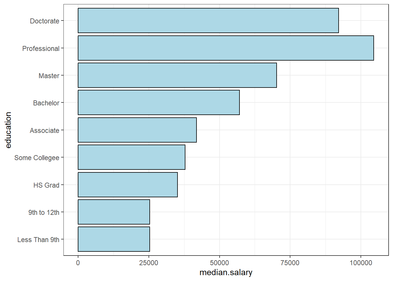
11.12 Current Population Survey, Incomes by Education

Current Population Survey. The Current Population Survey (CPS) is a monthly survey of thousands of U.S. households conducted by the United States Census Bureau for the Bureau of Labor Statistics (BLS). The BLS uses the data to publish reports early each month called the Employment Situation.

https://en.wikipedia.org/wiki/Current_Population_Survey

I will pull up the EXCEL spreadsheet for Both Sexes: 25 Years and Over: Total Work Experience: All Races and we will see data on incomes for people 25+ based on their level of educational attainment.

https://www.census.gov/data/tables/time-series/demo/income-poverty/cps-pinc/pinc-03.html

Here, I’ll just report the mean and median salaries by level of educational attainment (2018 data):

Level of Education	Mean Salary	Median Salary	Sample Size (with earnings)
Total	$60,131	$44,963	145,733
Less Than 9th Grade	$29,120	$25,318	3,744
9th to 12th Grade	$30,612	$25,280	6,282
High School Graduate (including G.E.D.)	$41,829	$35,016	36,668
Some college, no degree	$46,806	$37,811	22,517
Associate’s Degree	$49,966	$41,834	16,173
Bachelor’s Degree	$73,880	$57,105	37,449
Master’s Degree	$87,570	$70,241	16,784
Professional Degree	$150,215	$104,593	2,521
Doctorate Degree	$125,331	$92,126	3,606

1. Is this an observational study or a randomized experiment?

2. Do you think the mean or median is better for incomes?

3. Would you like to see this information provided in a graph?

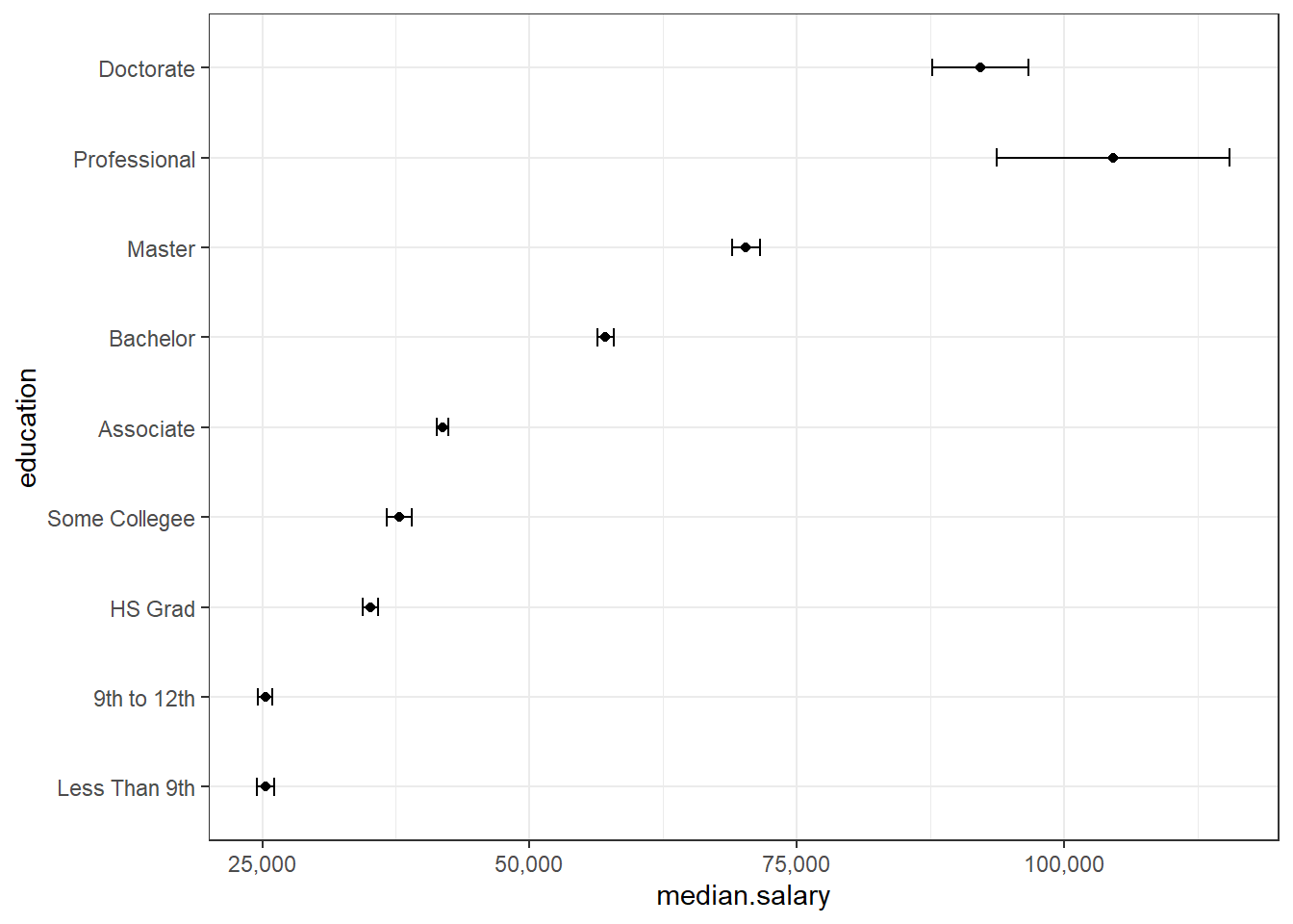
4. What is a “standard error”?

5. What pattern do you see in this data? Do you think this pattern would be statistically significant? Are these differences practically significant?

Here is a graph (visualization) of the data (using the medians and the standard error of the median).