Chapter 9 Multiple Regression

9.1 Sports Car Example

We aren’t going to calculate the equations for multiple regression models in class (i.e. models that use more than one \(X\) variable), but we’ll look a bit at how to use them.

9.2 Two Continuous \(X\) Variables

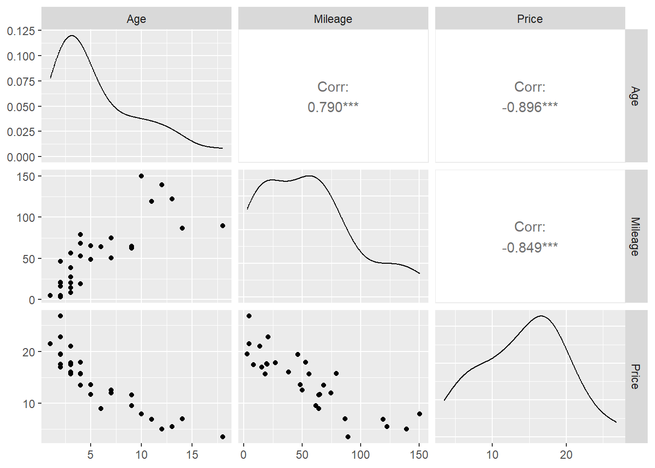
We’ll revisit the AccordPrices data set, where we will try to predict the Price of a used Honda Accord based on both Mileage and Age. I used software to create some graphs and to find the equation. The residual plot (i.e. the fitted values \(\hat{Y}\) on the \(x\)-axis and the residuals \(e\) on the \(y\)-axis) flares out like a horn or funnel, rather than just being a random assortment of points. This indicates more variability as the fitted value \(\hat{Y}\) increases (this is when the residuals are bigger).

\[\hat{Price} = 21.738 - 0.791Age - 0.053Mileage\]

## (Intercept)         Age     Mileage 
## 21.73825110 -0.79138059 -0.05314751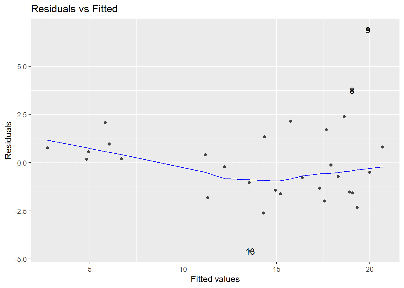

If I have a used Honda Accord that is 5 years old with 60,000 miles, I can predict its Price using Age\(=5\) and Mileage\(=60\).

\[\hat{Y}=21.738-0.791(5)-0.053(60)=14.603\]

The predicted price is about $14,600. If the actual price I sold it for was $13,000, then my residual would be \[e=Y-\hat{Y}=13-14.6=-1.6\] indicating I got about $1600 less than predicted (bad for me, good for the buyer).

9.3 One Continuous \(X\) and One Categorical \(X\)

Suppose a middle-aged man is having a mid-life crisis (not me, I didn’t buy a sports car) and is going to buy himself either a Jaguar or a Porsche. Suppose we want to predict its Price, based on both the cars’ Mileage (as before) and what type of Car he is going to buy.

Let’s look at a scatterplot, where different colors and shapes have been used to distinguish between Jaguars and Porsches.

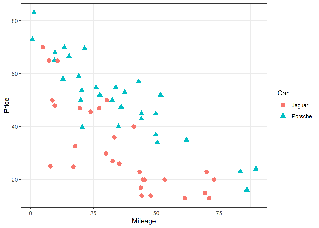
If I were to create two regression models, one to fit the Jaguars (the red circles) and another to fit the Porsches (the blue triangles), how do you think the two equations would be similar? How would they be different?

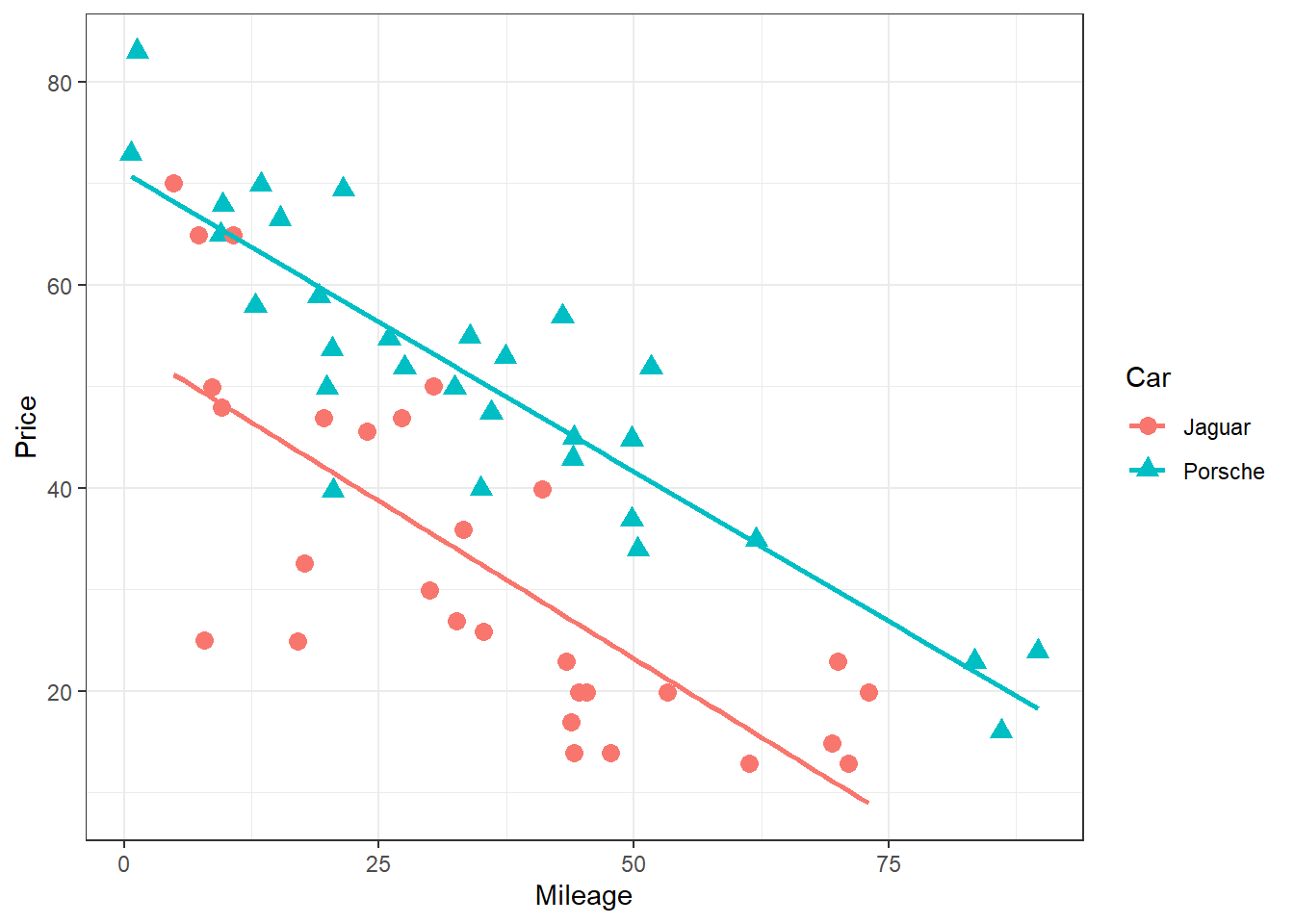
Below I’ve superimposed the regression lines for the two types of sports car on the plot.

If you guessed that the two lines would have different intercepts, which represents the Price when Mileage\(=0\), a new car, you were right.

If you also guessed that the two lines would have about the same slope, asthe blue and red lines are almost parallel, indicating both cars have a pretty similar rate of depreciation in Price as Mileage increases, you were right again.

Using statistical software, I can get a single equation to predict the price of a car, where CarPorsche\(=0\) represents a Jaguar and CarPorsche\(=1\) represents a Porsche.

## (Intercept)     Mileage  CarPorsche 
##   53.605550   -0.602977   17.958331

\[\hat{Price} = 53.606 - 0.603Mileage + 17.958CarPorsche\]

What does the positive coefficient \(17.598\) for Car represent? This is the difference in Price between a Jaguar and a Porsche when they have the same Mileage.

For a new car with Mileage=0 \[\hat{Y}_{Jaguar} = 53.606 - 0.603(0) + 17.958(0) = 53.606\] \[\hat{Y}_{Porsche} = 53.606 - 0.603(0) + 17.598(1) = 71.204\]