Chapter 15 Probability Models
We are only going to cover the binomial distribution (or probability model) and will not cover the geometric or Poisson models that are covered in the textbook.
15.1 Binomial Distribution
Suppose I flipped a coin \(n=3\) times and wanted to compute the probability of getting heads exactly \(X=2\) times. This can be done with a tree diagram.
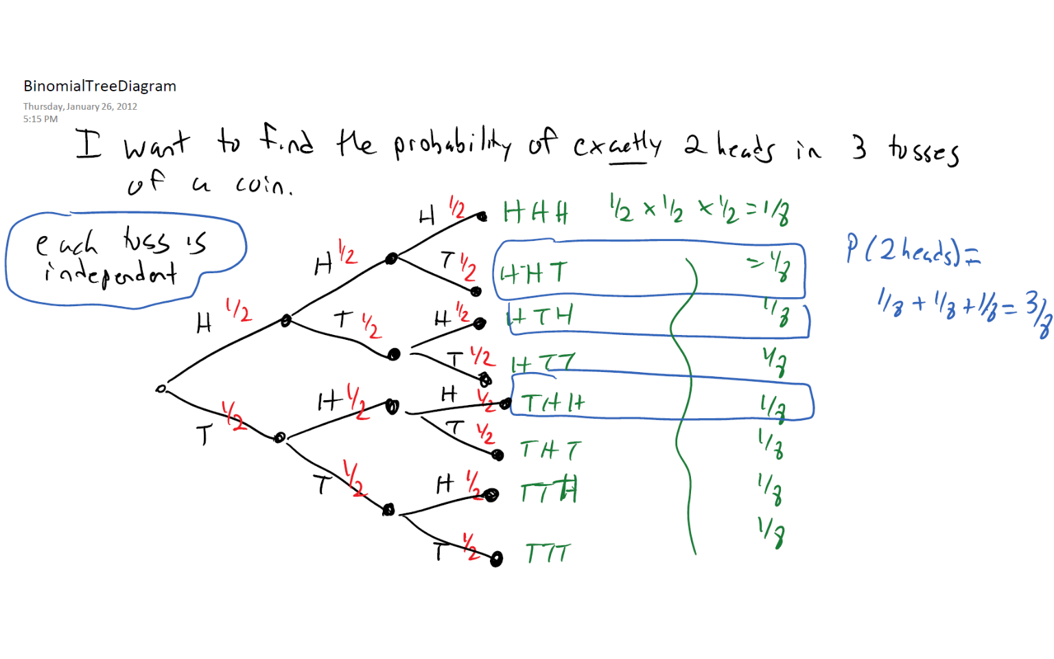
You can see that the tree diagram approach will not be viable for a large number of trials, say flipping a coin \(n=20\) times.
The binomial distribution is a probability model that will allow us to make computations such as the probability of getting \(X=12\) heads in \(n=20\) flips of a coin without constructing the tree diagram.
The binomial distribution is based on the assumption that we have Bernoulli trials, where:
- We have \(n\) independent trials of an event, such as flipping a coin 20 times.
- Each trial has two possible outcomes; one is a success (heads) and the other is failure (tails).
- The probability of success is known and the same for each trial; for coin flipping, \(p=0.50\).
15.2 Probability Density Function
The probability density function (p.d.f.) for the binomial distribution, for \(x=0,1,2,\ldots,n\), is:
\[P(X=x)={n \choose x} p^x (1-p)^{n-x}\]
where:
\(X\) is the random variable representing the number of successes
\(n\) is the number of trials
\(x\) is the observed number of successes
\(p\) is probability of success
\(n-x\) is the observed number of failures
\(1-p\) is the probabiity of failure (sometimes denoted as \(q\))
\({n \choose x}\) is \(n\) choose \(x\) (sometimes called the binomial coefficient)
\(n\) choose \(x\), which is usually represented as \({n \choose x}\) or \(_nC_x\), represents the number of ways to select \(x\) successes in \(n\) trials (without regard to order. and is computed as:
\[{n \choose x}=\frac{n!}{x!(n-x)!}\]
For example:
\[{4 \choose 3}=\frac{4!}{3! \times 1!}=\frac{4 \times 3 \times 2 \times 1}{3 \times 2 \times 1 \times 1}=4\]
If we are flipping a coin 4 times, there are 4 ways to get 3 heads: \(\{H,H,H,T\}, \{H,H,T,H\}, \{H,T,H,H\}, \{T,H,H,H\}\)
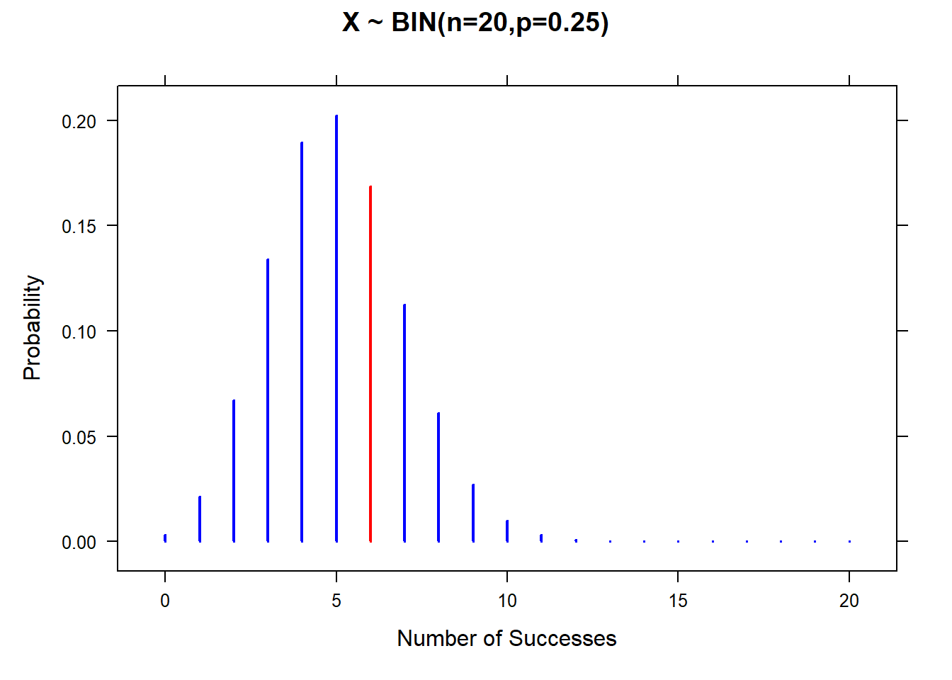
Suppose I take a \(n=20\) multiple choice test by guessing. Each question has 4 choices, one of which is correct. My probability of `success’ (guessing correctly) is \(p=0.25\). If \(X\) represents the number of correct answers, then \(X\) has a binomial distribution. \[X \sim BIN(20,0.25)\]
If I want to know the probability of getting exactly 6 questions right: \[P(X=6)={20 \choose 6}(0.25)^6 (0.75)^{14}=38760 (0.25)^6 (0.75)^{14}=.1686\]
These computations are tedious and difficult to perform without a calculator. The TI-83/84 calculator has functions to compute binomial probabilities, that remove the need to directly use the formula or have a special table.
With the calculator, go to \(\texttt{2nd, VARS,}\) and choose \(\texttt{Option A: binompdf}\), in the \(\texttt{DISTR}\) menu. The calculator expects one to enter \(\texttt{binompdf(n,p,x)}\), so \(\texttt{binompdf(20,0.25,6)=.1686}\), as seen before.
15.3 Cumulative Distribution Function
Often we want to know a cumulative probability, such as \(P(X \leq 6\) when \(X \sim BIN(n=20, p=0.25)\).
Literally, this is \(P(X \leq 6)=P(X=0)+P(X=1)+\cdots+P(X=5)+P(X=6)\).
This could be computed via using the probability density function (`formula’) several times.
\[P(X \leq 6)=.0032+.0211+.0669+.1339+.1897+.2023+.1686=.7857\]
The TI-83/84 calculator also has a function to compute binomial cumulative probabilities, using the cumulative distribution function or CDF.
With the calculator, go to \(\texttt{2nd, VARS,}\) and choose \(\texttt{Option B: binomcdf}\), in the \(\texttt{DISTR}\) menu. The calculator expects one to enter \(\texttt{binomcdf(n,p,x)}\), so \(\texttt{binomcdf(20,0.25,6)=.7858}\).
15.4 Other Inequalities
The simplest way to solve problems involving other inequalities besides less-than or equal to is to be `clever’ with the complement rule.
For example, if \(X \sim BIN(n=20,p=0.25)\) and we have already found that \(P(X=6)=.1686\) and \(P(X \leq 6)=.7858\), then:
\(P(X \neq 6)=1-P(X=6)=1-.1686=.8314\)
\(P(X<6)=P(X \leq 5)=.7858-.1686=.6172\)
\(P(X \geq 6)=1-P(X \leq 5)=1-.6172=.3823\)
\(P(X>6)=1-P(X \leq 6)=1-.7858=.2142\)
15.5 Mean and Variance of the Binomial
Many of the well-known probability distributions, including the binomial distributions, have what I like to call ‘short-cut’ formulas for finding the expected value and variance that is easier than the formulas seen previously for ‘generic’ discrete probability distributions.
For a binomial distribution, if \(X \sim BIN(n,p)\), then: \[\mu_X=E(X)=np\] \[\sigma^2_X=Var(X)=np(1-p)\]
So if \(n=20\) and \(p=0.25\), then \[\mu_X=E(X)=20(.25)=5\] \[\sigma^2_X=Var(X)=20(.25)(.75)=3.75\] \[\sigma_X=SD(X)=\sqrt{3.75}=1.936\]