Chapter 17 Confidence Interval for a Mean
17.1 Sampling Distribution of the Sample Mean
- Suppose I roll five 6-sided dice and take the average (i.e. \(\bar{x}\)) of the dice rolls. For instance, if I got (3,2,6,2,4), then \(\bar{x}=\frac{17}{5}\). We could repeat rolling and averaging 5 dice thousands of times and graph the results.
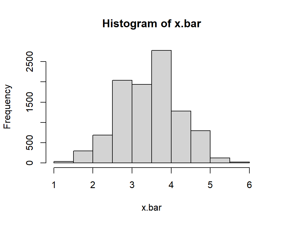
## [1] 3.49688## [1] 0.7653345The mean of the uniform distribution based on rolling a single die is: \[\mu_X=E(X)=\frac{m+1}{2}\]
With \(m=6\), \(\mu_X=3.5\).
The standard deviation of the uniform distribution is: \[\sigma_X=SD(X)=\sqrt{\frac{m^2-1}{12}}\].
With \(m=6\), \(\sigma_X=\sqrt{\frac{35}{12}}=1.708\)
The mean of the sampling distribution of the means is: \[\mu_{\bar{X}}=\mu_X\] (i.e. the same as the original mean of the population)
The standard deviation of the sampling distribution of the means (which we will call the standard error) is:
\[\sigma_{\bar{X}}=\frac{\sigma_X}{\sqrt{n}}\]
Notice this is NOT the same as the standard deviation of the population; it gets smaller as \(n\) increases. In our case the standard error is \(\sigma_{\bar{X}}=\frac{1.708}{\sqrt{5}}=0.764\).
17.2 The Central Limit Theorem
The fundamental theorem of statistics is the Central Limit Theorem (CLT).
Central Limit Theorem: Draw many, many random samples of size \(n\) from some population (which may or may not be normal). If the sample size \(n\) is ‘large’ enough, then the sampling distribution of the sample mean \(\bar{x}\) will be approximately normal.
\[\bar{X} \dot{\sim} N(\mu_{\bar{X}}=\mu, \sigma_{\bar{X}}=\frac{\sigma}{\sqrt{n}})\]
17.3 The CLT in a Best Case Scenario
Suppose the amount of liquid, in ML, in a bottle of Diet Pepsi follows a normal distribution \(X \sim(\mu=593, \sigma=1.4)\). Since \(X\) is normal, then \(\bar{X}\) will be normal for any sample size \(n\).
Finding \(P(X<591)\) for a single bottle of Pepsi is just a normal curve problem, solvable with a normal table or the normalcdf function on the calculator.
\(Z=\frac{591-593}{1.4}=-1.43\)
We saw in class that \(P(X<591)=P(Z<-1.43)=0.0764\) with table, or normalcdf(-1E99,591,593,1.4)=0.0766 with the calculator.
If we take a sample of \(n=10\) bottles, then \(\sigma_{\bar{x}}=\frac{1.4}{\sqrt{10}}\).
\(Z=\frac{591-592}{1.4/\sqrt{10}}=-4.52\)
\(P(\bar{X}<591)=P(Z<-4.52)\), which is virtually zero.
With the calculator, normalcdf(-1E99,591,593,1.4/sqrt(10))=3.13106054E-06, which is \(3.13 \times 10^{-6}=0.00000313\).
17.4 The CLT in a Worst Case Scenario
If the distribution of \(X\) is unknown or known to be skewed, then \(n \geq 30\) for the sampling distribution to be approx. normal.
Example #1 (Survival Times–Heavily Skewed):
The lifetime of a certain insect could be described by an exponential distribution with mean \(\mu=1000\) hours and standard deviation \(\sigma=1000\) hours. This distribution is heavily skewed and non-normal. This particular continuous distribution is sometimes used to model survival times when deaths/failures happen randomly. More advanced distributions (such as the Weibull) can more accurately model survival when deaths/failures do not occur randomly. When most deaths/failures occur early, an ‘infant-mortality’ model is used, while if most deaths/failures occur later, an ‘old-age wearout’ model is used.
Suppose I want to find \(P(X>1100)\). We cannot (with MAT 135 level methods) find this probability, and a normal approximation would be terrible!
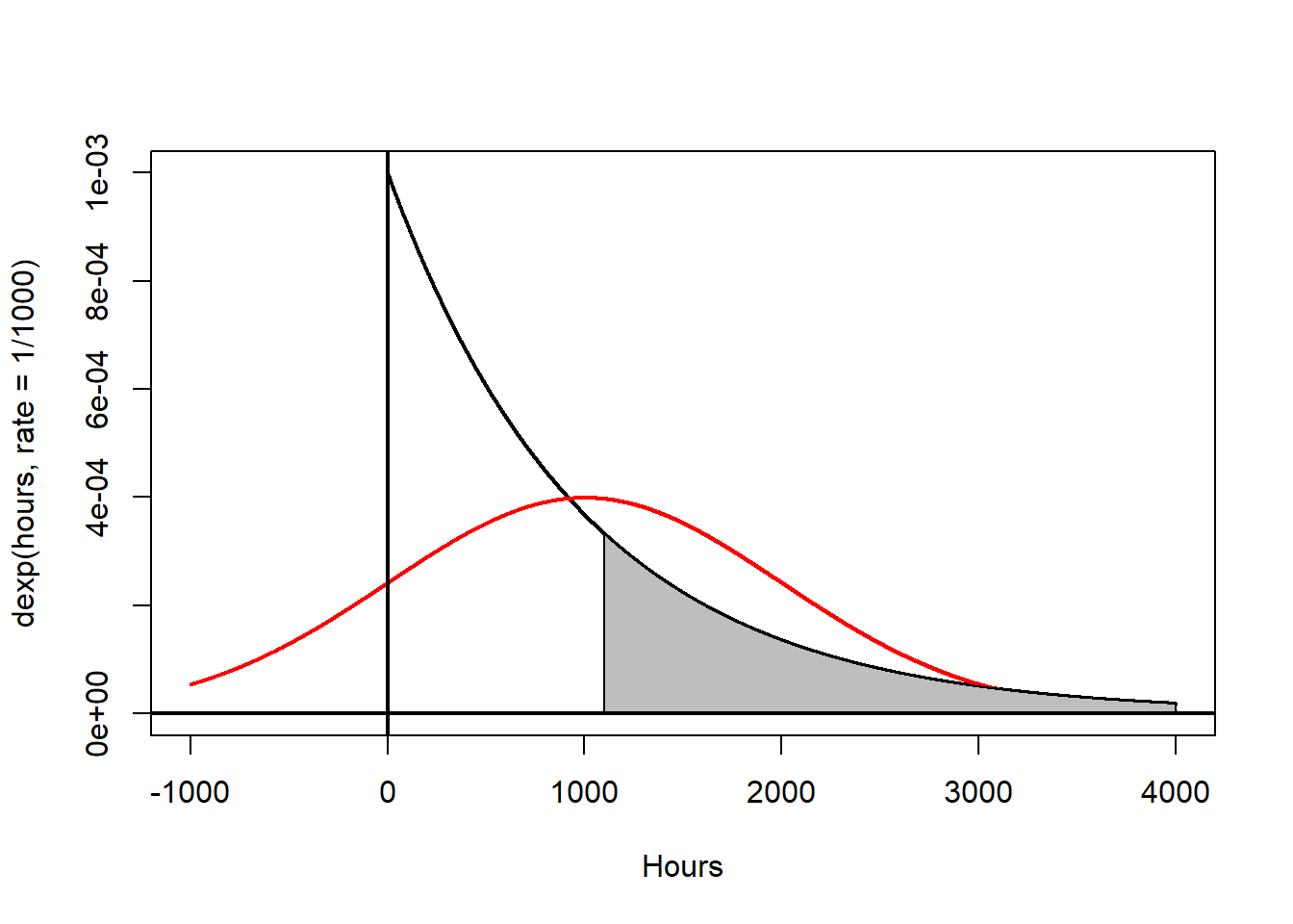
However, using the Central Limit Theorem, we can compute \(P(\bar{X}>1100)\) for a sample of \(n=30\) insects.
I will simulate the sampling distribution and draw its histogram, superimposing a normal curve with mean \(\mu_{\bar{x}}=1000\) and standard error \(\sigma_{\bar{x}}=\frac{1000}{\sqrt{30}}=\) 182.5741858 on top of it.
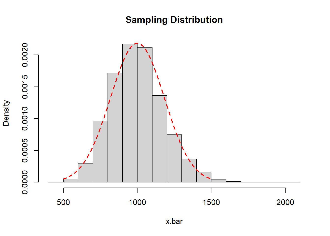
The sample mean of my sampling distribution is 999.0773615 and the standard deviation of my sampling distribution (standard error) is 180.4848471. these are close to the theoretical values.
So \(P(\bar{X}>1100)\) for a sample of \(n=30\) is just another normal curve problem based on \(\bar{X} \dot{\sim} N(1000,1000/\sqrt{30})\).
\(Z=\frac{\bar{X}-\mu}{\sigma/\sqrt{n}}=\frac{1100-1000}{1000/\sqrt{30}}=\) 0.55
\(P(Z>0.55)=1-0.7088=.2912\)
Or with the TI: normalcdf(1100,1E99,1000,182.5742)=.2919
Example #2 (Baseball Salaries-Heavily Skewed : The beauty of the Central Limit Theorem is that even when we sample from a population whose distribution is either unknown or is known to be some heavily skewed (and very non-normal) distribution, the sampling distribution of the sample mean \(\bar{X}\) is approximately normal when \(n\) is ‘large’ enough. Often \(n > 30\) is used as a Rule of Thumb for when the sampling distribution will be large enough.
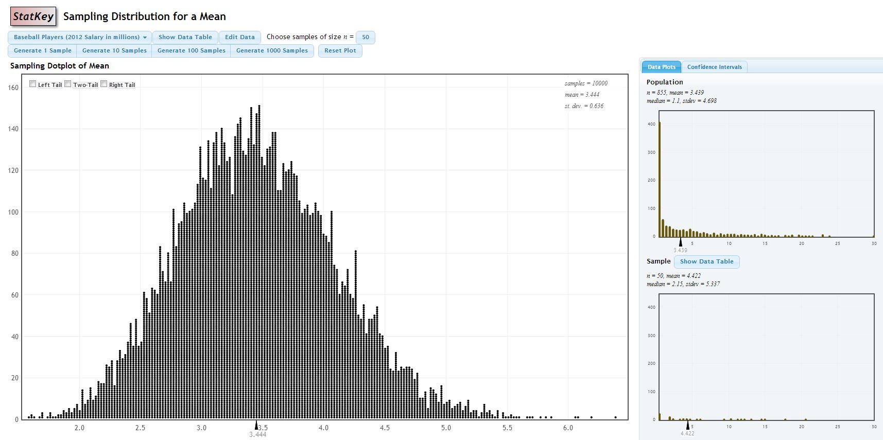
A nice online demonstration of this can be found at (http://www.lock5stat.com/statkey/index.html). At this site, go to Sampling Distribution: Mean link (about the middle of the page or directly at http://www.lock5stat.com/statkey/sampling_1_quant/sampling_1_quant.html). In the upper left hand corner, change the data set to Baseball Players-this is salary data for professional baseball players in 2012. On the right hand side, you see that the population is heavily right-skewed due to a handful of players making HUGE salaries.
You can choose samples of various sizes–the default is \(n=10\) and generate thousands of samples. The sample mean \(\bar{X}\) is computed for each sample and the big graph in the middle of the page is the sampling distribution. Notice what happens to the shape of this distribution, along with the mean and the standard error of the sampling distribution.
The original population of \(n=855\) players is heavily skewed and non-normal with mean \(\mu=3.439\) million dollars (wow!) and \(\sigma=4.698\) million. I will take 10000 samples, each of size \(n=50\).
Baseball
The mean of the sampling distribution of \(\bar{X}\) is \(3.444\), which is very close to \(\mu\) for the population.
The standard error of the sampling distribution is \(0.636\). Theoretically, it should be \(\sigma_{\bar{X}}=\frac{\sigma}{\sqrt{n}}=\frac{4.698}{\sqrt{50}}=0.664\), again very close.
The shape is approximately normal (although a bit of skew is still visible).
17.5 Confidence Interval for a Mean, Based on \(z\) distribution
Suppose we want a \(100(1-\alpha)\%\) confidence interval for a mean. If we assume \(X \sim N(\mu, \sigma)\) where the value of \(\sigma\) is known, then \(\bar{X} \sim N(\mu, \sigma/\sqrt{n})\). So the formula will be:
\[\bar{x} \pm z^* \times \frac{\sigma}{\sqrt{n}}\]
This is basically identical to our formula for the CI of a proportion, substituting \(\bar{x}\) for \(\hat{p}\) as the point estimte and \(\frac{\sigma}{\sqrt{n}}\) for \(\sqrt{\frac{\hat{p} \hat{q}}{n}}\) as the standard error.
It might have struck you as strange that we would know the true standard deviation \(\sigma\) of a distribution in a situation where we did not know the true mean \(\mu\) and felt it necessary to estimate \(\mu\) with a point estimate \(\bar{x}\) and a confidence interval.
In most situations, we would not know the true value for \(\sigma\). The sample standard deviation \(s\) seems like a natural choice to use in place of \(\sigma\) in our confidence interval formulas.
However, the distribution of the quantity \(\frac{\bar{x}-\mu}{s/\sqrt{n}}\) does not precisely follow a normal distribution, especially when \(n\) is small. The sampling distribution in this case follows the \(t\)-distribution, discovered by William Gosset.
17.6 The \(t\)-distribution
The \(t\)-distribution is similar to the standard normal distribution in that it is:
- Bell-shaped
- Symmetric
- Has \(\mu=0\)
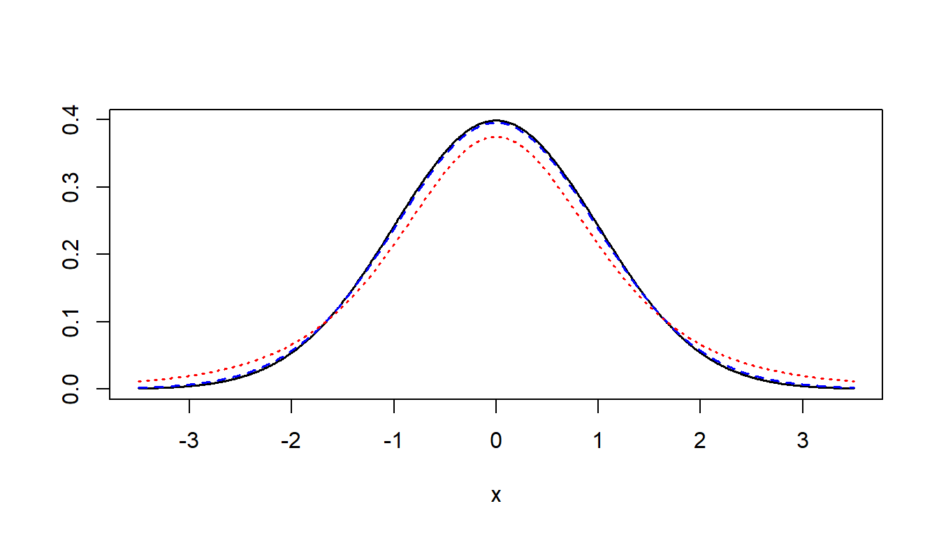
However, the \(t\)-distribution has ‘heavier tails’ (i.e. a higher variance) than the standard normal distribution. Visually, it is shorter and flatter than the standard normal curve, as seen on the next slide. Also, each \(t\) distribuiton is dscribed by a parameter called degrees of freedom, where \(df=n-1\). As \(n \rightarrow \infty\), the \(t\)-curve approaches the \(z\)-curve.
The black line is standard normal, the blue line (very close to the black) is \(t\) with 30 df, and the red line (further from the black) is \(t\) with 4 df.
17.7 Confidence Interval Based On the \(t\) distribution
The formula for the confidence interval for a mean is changed slightly when we do not know \(\sigma\). We still need to assume \(X\) follows a normal distribution, or that we have a large sample size (\(n>30\)).
\[\bar{x} \pm t^* \times \frac{s}{\sqrt{n}}\]
We need to know both \(n\) and \(\alpha\) to find the critical value \(t^*\). The degrees of freedom are \(df=n-1\) and the critical value will change for each sample size.
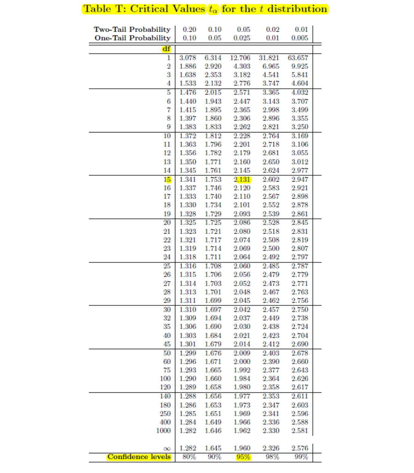
If \(df=15\) and a 95% confidence level (\(\alpha=.05\)), then we can use a \(t\)-distribution table such as the one in the textbook. Use the row with \(df=15\) and the column with a confidence level of 95% (read from the bottom of the table). The critical value is \(t^*=\pm 2.131\).
If \(n=16\) (so \(df=15\)), \(\bar{x}=192.4\) and \(s=26.5\), then the 95% confidence interval for \(\mu\) is:
\[192.4 \pm 2.131 \times \frac{26.5}{\sqrt{16}}\]
\[192.4 \pm 14.12\]
The \(t\) critical value can be obtained with technology. Use invT(.025,15) and invT(.975,15) on a TI calculator. You should still get \(t=\pm2.131\).
Or, use 8:TInterval from the TESTS menu.