Chapter 18 Testing Hypotheses

18.1 The One Proportion \(z\)-test

In chapter 18, we will study our first examples of hypothesis tests. The first will be a procedure known as the One-Proportion \(Z\)-test. As you will see, it is closely related to the confidence interval for a proportion \(p\) studied in chapter 16.

18.2 Six Step Method for Hypothesis Testing

I will be presenting hypothesis testing via a systematic six step process, and will expect you to use these steps when you work problems. I will work through our first example slowly and in great detail, since there is a lot of new concepts and terminology to discuss.

Step One: Write Hypotheses

For our first example, suppose that we have a coin that we suspect is unfair (i.e. the coin will not give us heads 50% of the time if we flip it many times). This research question will be turned into a pair of mathematical statements called the null and alternative hypotheses. Hypotheses are statements about the value of a parameter, not a statistic.

The null hypothesis, or \(H_O\), states that there is no difference (or effect) from the population parameter (hypothesized value) and is what will be statistically tested. The alternative hypothesis, or \(H_A\), states that there is some sort of difference (or effect) from that parameter. The alternative will typically correspond to one’s research hypothesis.

\[H_O: p=0.50\]

\[H_A: p \neq 0.50\]

For our artificial first example, the null hypothesis is stating that our coin is fair (gives heads 50% of the time), while the alternative hypothesis is stating that the coin is unfair and does not give heads 50% of the time. This is an example of a two-sided hypothesis, also called a non-directional hypothesis. It is two-sided (non-directional) because we have NOT indicated any sort of a priori belief that the coin was biased to give either more than 50% or fewer than 50% heads when flipped.

In many research situations, we will have a one-sided or directional hypothesis. For example, a medical study might look to see if a treatment will significantly lower the average blood pressure of patients when compared to a control. I will illustrate both possible directions, first if we think the coin is biased in favor of heads.

\[H_O: p=0.50\]

\[H_A: p>0.50\]

Next, consider if we thought the coin was biased in favor of tails.

\[H_O: p=0.50\]

\[H_A: p<0.50\]

Step Two: Choose Level of Significance

This is where you choose your value for \(\alpha\) (usually 0.05), thereby setting the risk one is willing to take of rejecting the null hypothesis when it is actually true (i.e. declaring that you found a significant effect that in fact does not exist).

\[\alpha=0.05\]

A two-sided hypothesis test at level \(\alpha\) will correspond to a \(100(1-\alpha)\%\) confidence interval.

Step Three: Choose Your Test and Check Assumptions This is where you choose your ‘tool’ (i.e. test) and check the mathematical assumptions of that test to make sure you are using the proper ‘tool’ for the job. For the one-proportion \(z\)-test, the assumptions are:

the data is from a random sample
the data values are independent
the sample size is sufficient to use the normal approximation to the binomial

Checking the first two conditions involves judging whether or not the sampling was done in a random and independent fashion. The third condition can be judged mathematically.

Suppose we plan on flipping the coin \(n=400\) times. These flips will clearly be random and independent. We can check to make sure that both the expected number of successes AND the expected number of failures are at least 10; check that \(np_O \geq 10\) and \(nq_0 \geq 10\). In our example, \(n=400\), \(p_O=0.5\) and \(q_O=1-p_O=1-0.5=0.5\), so we have 200 expected successes and 200 expected failures, more than enough, and we may proceed.

Step Four: Calculate the Test Statistic This is what you thought stats class was all about. You will use a formula (or an appropriate function on a calculator or software package) to compute a test statistic based on observed data. The test statistic for this test is:

\[z = \frac{\hat{p}-p_O}{\sqrt{\frac{p_O q_O}{n}}}\]

Suppose we obtain \(X=215\) heads in \(n=400\) flips, such that \(\hat{p}=\frac{215}{400}=0.5375\). Our test statistic will be:

\[z = \frac{.5375-.5}{\sqrt{\frac{0.5(0.5)}{400}}}=\frac{0.0375}{0.025}=1.5\]

The distribution of this test statistic \(z\) will be \(z \sim N(0,1)\) (i.e. standard normal) WHEN the null hypothesis is true.

Step Five: Make a Statistical Decision This is where you either determine the decision rule (‘old-school’) or compute a \(p\)-value (‘new-school’) and decide whether to reject or fail to reject the null hypothesis.

Step Five: Make a Statistical Decision (via the Decision Rule)

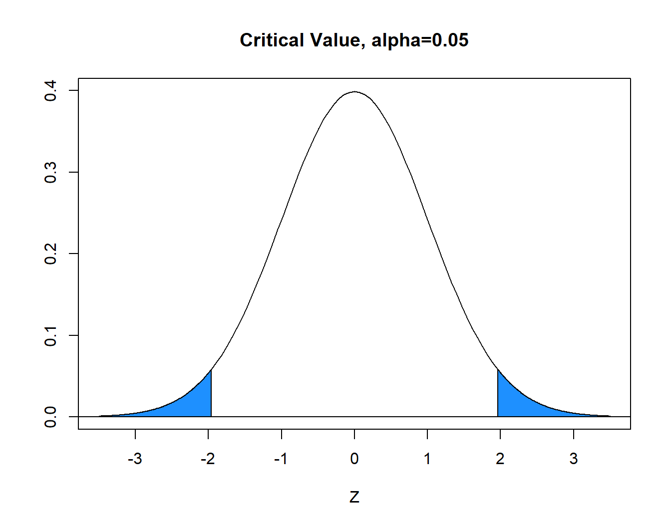
With \(\alpha=0.05\) (area in blue), the critical value is \(z^*=1.96\). The blue tails in the graph below each have area=\(\alpha/2=.025\) and the white area between is equal to \(1-\alpha=0.95\). Hence, the decision rule is to reject \(H_0\) when the absolute value of the computed test statistic \(z\) exceeds critical value \(z^*\), or reject \(H_0\) if \(|z|>z^*\). In our problem, \(|z|=1.50 \not > 1.96=z^*\) and we FAIL TO REJECT the null.

Step Five: Make a Statistical Decision (via the \(p\)-value)

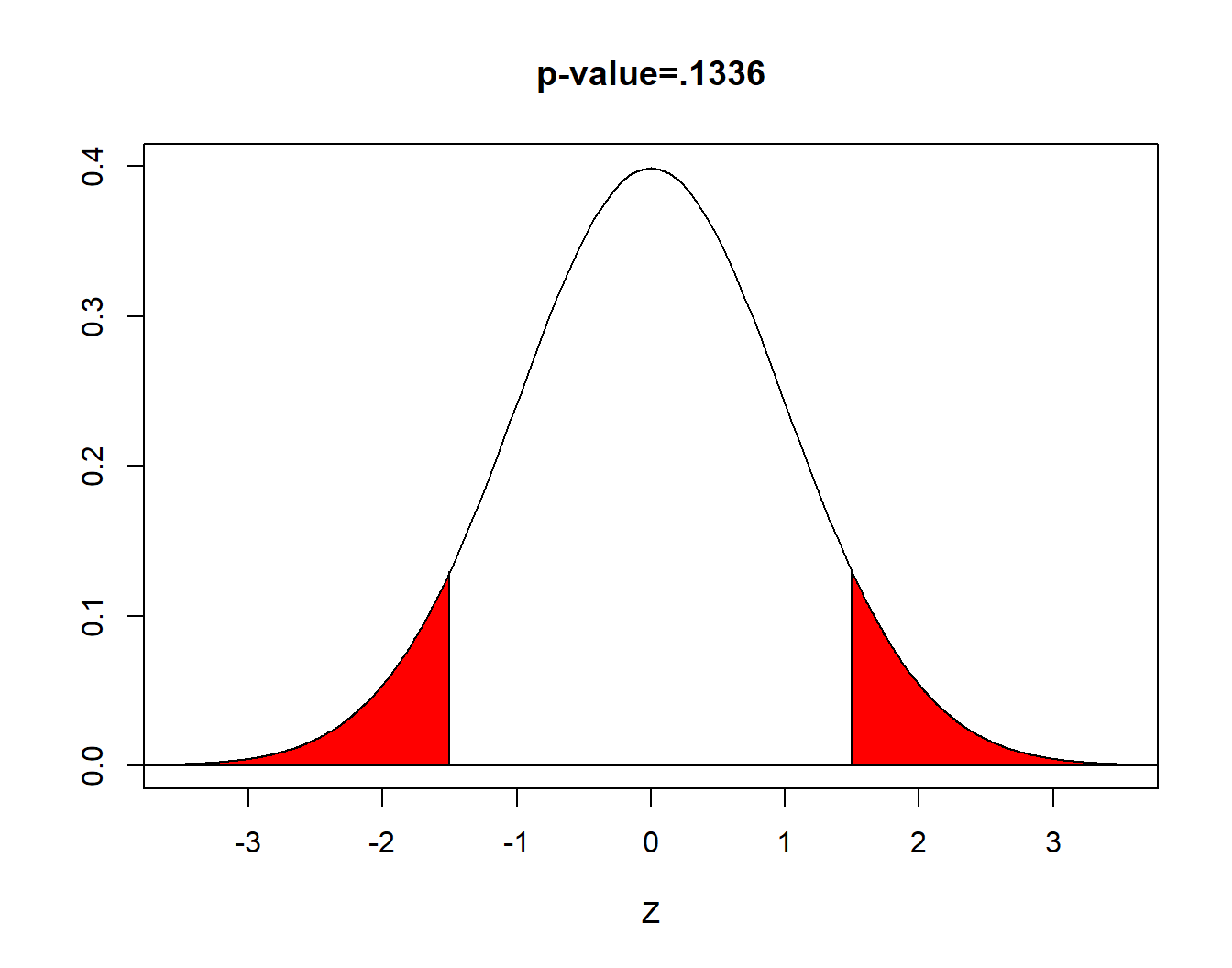
When you use technology, a statistic called the p-value will be computed, based on your computed test statistic. The \(p\)-value is defined to be the probability of obtaining a value as extreme as our test statistic, IF the null hypothesis is true. For our two-sided \(z\)-test,

\[ \begin{aligned} \text{p-value}= & P(|z|>1.50) \\ = & 2 \times P(z<-1.50) \\ = & 2 \times P(z>1.50) \\ = & 2 \times 0.0668 \\ = & 0.1336 \end{aligned} \] (area in red)

When the \(p\)-value is less than \(\alpha\), we reject the null hypothesis. We have ‘evidence beyond a reasonable doubt’.
When the \(p\)-value is greater than or equal to \(\alpha\), we fail to reject the null. We do not have ‘evidence beyond a reasonable doubt’.

Here \(.1336>.05\) and we fail to reject the null hypothesis

Step Six: Conclusion This is where you explain what all of this means to your audience. The terminology you use should be appropriate for the audience.

Since we rejected the null hypothesis, a proper conclusion would be:

The proportion of coin flips that are heads is NOT significantly different than 0.50. In other words, we do not have evidence to show the coin is unfair.

Remember, the amount of statistical jargon that you use in your conclusion depends on your audience! If your audience is a committee of professors, you can use more terminology than if your audience is someone like a school principal or hospital administrator or the general public.

18.3 Relationship Between a Two-Sided Test and a CI

In our problem, we computed \(z=1.50\) with \(p=.1336\) and rejected the null hypothesis at \(\alpha=0.05\). Suppose we computed the \(100(1-\alpha)\%\) confidence interval for a proportion for the coin flips data. Here, it is a 95% CI:

\[ 0.5375 \pm 1.96 \times \sqrt{\frac{.5375(1-.5375)}{400}}\] \[0.5375 \pm 0.0249\]

The 95% CI is \((0.5126,0.5624)\). The margin of error is \(\pm 2.49\%\) Notice the entire interval lies above the null value of \(p=0.50\) . This also leads to a failure to reject the null hypothesis (that the coin was fair).

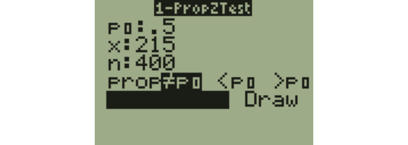
18.4 The One Proportion \(Z\)-test with technology

With a TI-83/84, go to STAT, then TESTS, and choose A:1-PropZInterval.

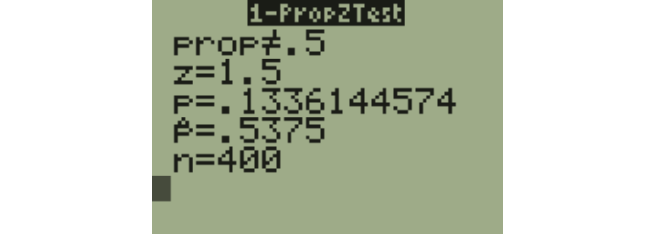
The results on our calculator agree with our earlier calculation.

18.5 What if We Have a One-Sided Test?

Suppose your original research hypothesis was that the coin was more likely to land on heads. Step One would change.

\[H_O: p=0.50\]

\[H_A: p > 0.50\]

Steps Two, Three, and Four will not change!

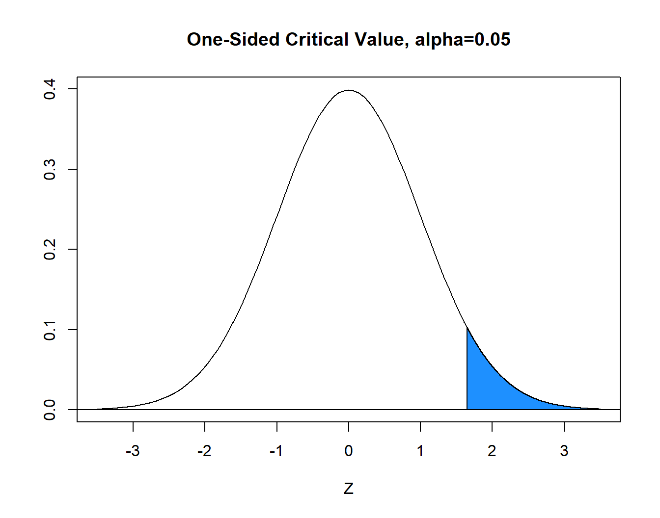
Step Five will change. If you are looking up the critical value \(z^*\) from the table to determine the decision rule, the entire area \(\alpha=.05\) will be on the right (or left) hand side of the normal curve. The critical value is \(z^*=1.645\), so reject \(H_0\) if \(z>1.645\).

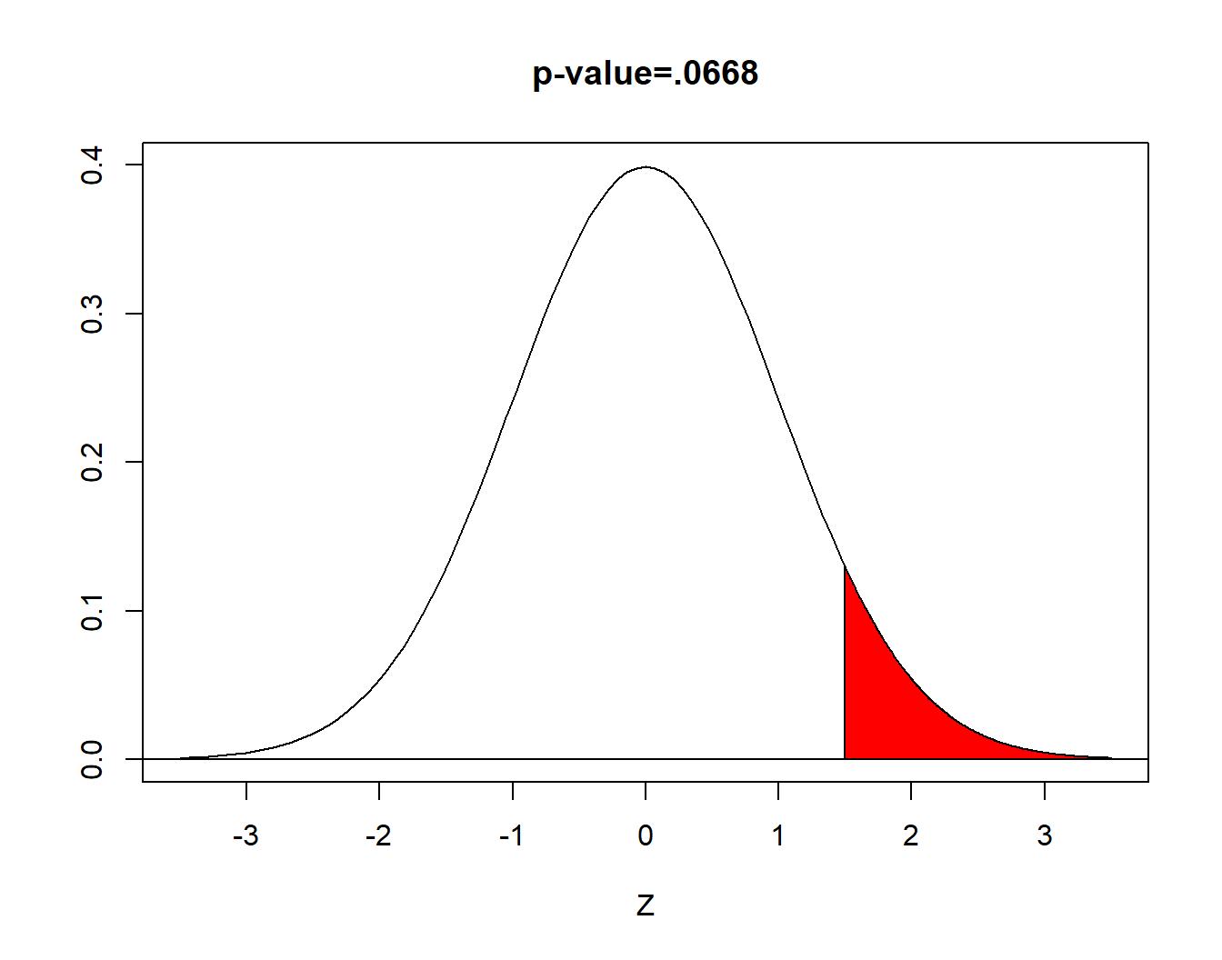
Step Five will change. If you are computing the \(p\)-value, it will only be the area to the right (or left) of the computed test statistic. In our problem, \(\text{p-value}=P(z>1.50)=.0668\). The \(p\)-value will be exactly half of what it was with the two-sided test on the same data.

We still fail to reject; step six will be slightly different:

The proportion of coin flips that are heads is NOT significantly greater than 0.50. In other words, we do not have evidence to show the coin is unfair or biased towards heads.

18.6 The \(t\)-test for a Single Mean

If the data were normally distributed and \(\sigma\) was known, we could use the test statistic

\[z=\frac{\bar{x}-\mu_O}{\sigma/\sqrt{n}}\]

Since \(\sigma\) will almost always be known, we will not conisder the \(z\)-test and instead will compute a test statistic

\[t=\frac{\bar{x}-\mu_O}{s/\sqrt{n}}\]

This statistic will follow a \(t\)-distribution with \(df=n-1\) when the null is true, and we will determine the decision rule and the \(p\)-value based on that \(t\)-distribution.

Example: The One-Sample \(t\)-test

Suppose we have a sample of \(n=16\) seven-year-old boys from Kentucky. We have a hypothesis that these boys will be heavier than the national average of \(\mu=52\) pounds. We will not assume that we have ‘magical’ knowledge about the value of \(\sigma\) or whether this data is normally distributed or not.

Since we are not assuming that the variance is known, the \(z\)-test is not the proper ‘tool’ (and we will ignore 1:ZTest in the TI Tests menu); we will reach into our toolbox and use the one-sample \(t\)-test instead (which is 2:TTest).

Step One: Write Hypotheses

\[H_0: \mu=52\] \[H_a: \mu > 52\]

Step Two: Choose Level of Significance

Let \(\alpha=0.05\).

Step Three: Choose Test & Check Assumptions

Suppose the \(n=16\) data values are: \[48 \quad 48 \quad 48 \quad 60 \quad 48 \quad 45 \quad 57 \quad 46\] \[95 \quad 53 \quad 53 \quad 64 \quad 57 \quad 53 \quad 60 \quad 55\]

One boy seems to be an outlier. Maybe he is obese or very tall for his age. This data point might cause the distribution to be skewed and affect our ability to use the \(t\)-test!

Checking for Normality

One of the mathematical assumptions of the \(t\)-test is that the data is normally distributed. If we have a large sample, \(n>30\), the Central Limit Theorem states that the sampling distribution of \(\bar{x}\) will be approx. normal. We do not have a large sample.

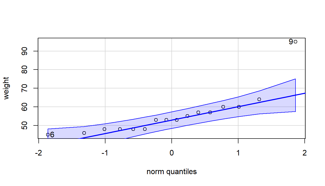
The normal probability plot, or QQ-plot, is a graphical test for normality and can be made with the STATPLOT menu on a calculator

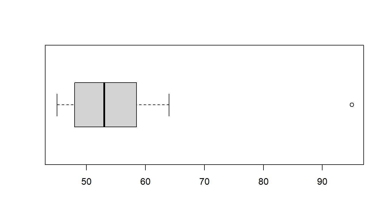
In practice, we can `bend the rules’ a bit and use the \(t\)-test as long as the data is close to symmetric and not heavily skewed with outliers. A boxplot can be used to check for this, which is easier to interpret. I have constructed both plots with software and we’ll do so with the calculator in class.

If the data is normally distributed, the points in the qq-plot should fall close to a straight line and all should be inside the dashed arcs. Our heavy boy, \(x=95\), in the upper right hand corner falls well outside and is ‘skewing’ the distribution.

## [1] 9 6

A simpler plot to understand is the boxplot. The heavy boy (boy #9) shows up as an outlier, which we do not want to see if we are planning on using a \(t\)-test with a small data set.

18.7 What about outliers?

Most statisticians do not consider it appropriate to delete an outlier unless there is both a statistical and a non-statistical reason for that deletion. Outliers can occur for several reasons: there might have been a data entry error (maybe that 95 was really 59), that observation might not belong to the population (maybe that boy was actually 11 years old), or it might be a true observation (that boy is obese and/or very tall for his age).

For our example, it was a data entry error. The boy was actually 59 pounds. The QQ plot and boxplot are fine when the point is corrected.

\[48 \quad 48 \quad 48 \quad 60 \quad 48 \quad 45 \quad 57 \quad 46\] \[59 \quad 53 \quad 53 \quad 64 \quad 57 \quad 53 \quad 60 \quad 55\]

Back to our One-Sample \(t\)-test

In order to do Step Four and compute the test statistic, we need the sample mean and standard deviation of the weights. With the corrected value of 59, we get \(\bar{x}=53.375\), \(s=5.784\), \(n=16\).

Step Four: Calculate the Test Statistic

\[t=\frac{\bar{x}-\mu_0}{s/\sqrt{n}}\]

\[t=\frac{53.375-52}{5.784/\sqrt{16}}=\frac{1.375}{1.446}=0.951\]

\[df=n-1=16-1=15\]

Step Five: Make a Statistical Decision (via the Decision Rule)

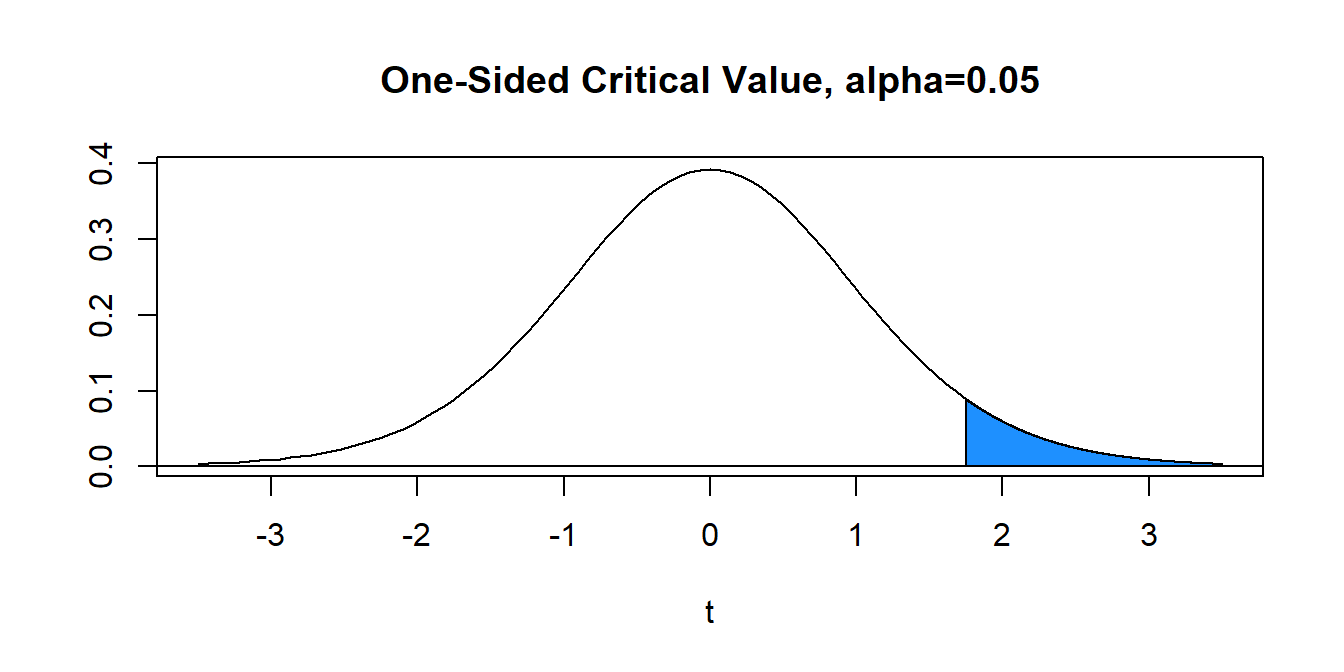
With \(\alpha=0.05\) (area in blue) and \(df=15\), the critical value is \(t^*= 1.753\). Hence, the decision rule is to reject \(H_0\) when the value of the computed test statistic \(t\) exceeds critical value \(t^*\), or reject \(H_0\) if \(t>t^*\). In our problem, \(t=0.951 \not > 1.753=t^*\) and we FAIL TO REJECT the null.

Step Five: Make a Statistical Decision (via the \(p\)-value)

Computation of the \(p\)-value will be more difficult for us with the \(t\)-test than the \(z\)-test. The reason is that the \(t\)-table that is generally provided in statistical textbooks is much less extensive than the standard normal table. For us to be able to compute the exact \(p\)-value for a \(t\)-test, we need to:

Have a two page \(t\)-table similar to the normal table for every possible value of \(df\); that is, every row of the \(t\)-table would become two pages of probabilities. We do not have access to such tables. We can approximate the \(p\)-value with our one-page \(t\)-table.
Evaluate the integral \(P(t>0.951)=\int_{0.951}^{\infty} f(x) dx\), where \(f(x)\) is the probability density function for the \(t\)-distribution with \(n-1\) df. If you aren’t a math major, this may sound scary and awful! If you are a math major, you know this is scary and awful! So we won’t do it!
Use techonology to get the \(p\)-value; that is, let the calculator or computer do the difficult math needed to compute the \(p\)-value.

In our problem, we have the one-sided alternative hypothesis \(H_a: \mu > 52\), a test statistic \(t=0.951\), and \(df=15\).

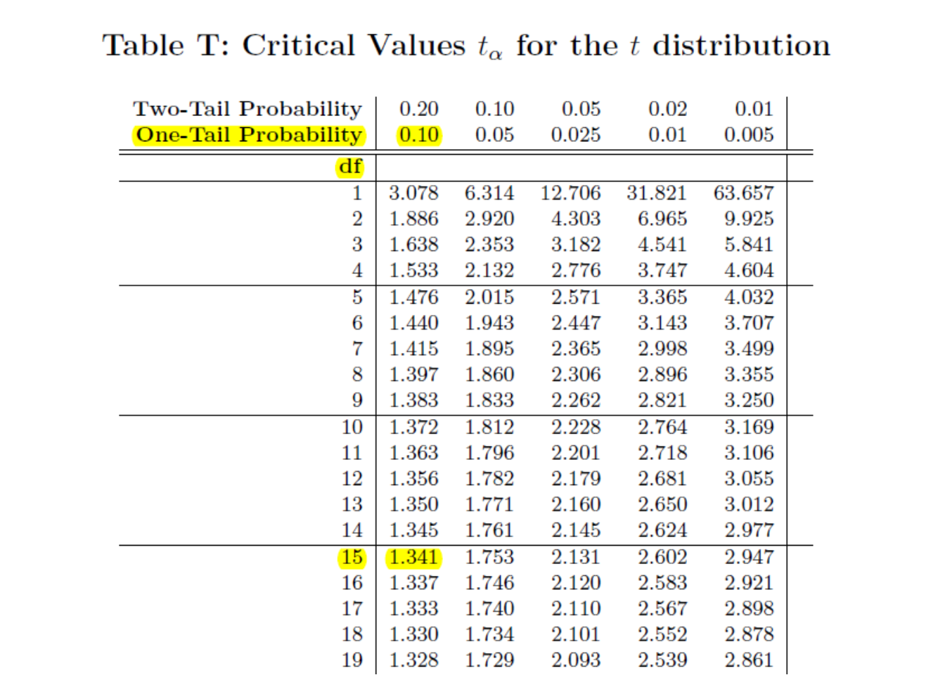
Below shows a \(t\)-table with the pertinent values highlighted. We refer to the row for \(df=15\). Notice our test statistic \(t=0.951\) falls below the critical values \(t^*=1.341\).

The area above \(t^*=1.341\) is .10. Hence, our \(p\)-value is greater than .10, or \(\text{p-value}>.10\). If we had \(H_a: \mu \neq 52\), then it would be \(\text{p-value}>.20\).

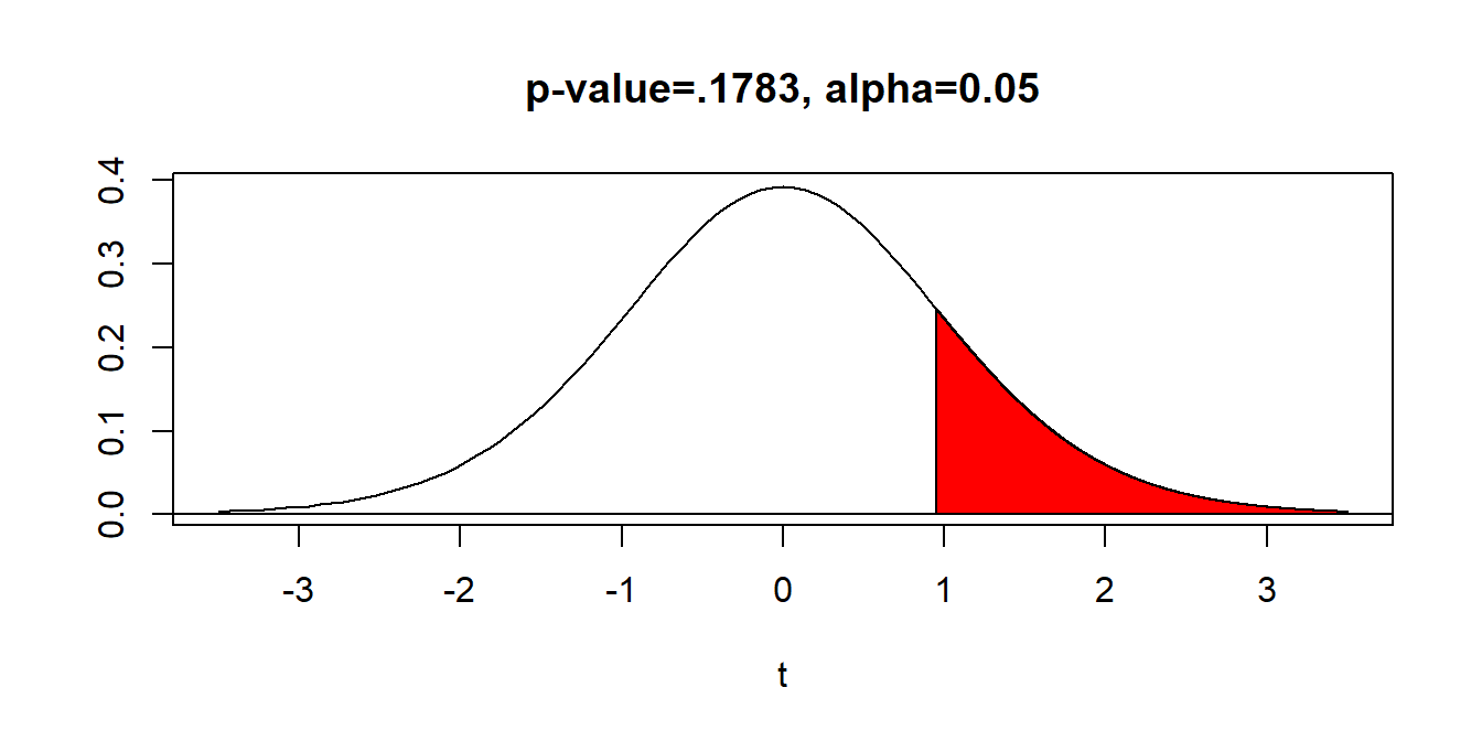
The \(p\)-value can be obtained with technology. Use tcdf(0.951,999999999,15) on a TI calculator. You should get \(p=0.1783\).

Step Six: Conclusion

Since we failed to reject the null hypothesis, a proper conclusion would be:

The mean weight of seven-year-old boys in Kentucky is NOT significantly greater than the national average of 52 pounds.

On the TI-83/84, go to STAT, TESTS, 2:T-Test... (screen shots on the next few slides)

On the calculator, assume that the boys’ weights have been entered in List L1.

Here are the results