Chapter 20 Comparing Independent Groups
20.1 Independent Samples \(t\)-test
Here, we will cover how to test a hypothesis involving independent samples (also called the two-sample \(t\)-test). This is when we take measurements on subjects from two groups that are independnet of each other, to see if some sort of significant change has occurred.
Difference of Two Independent Means
Often we want to test the difference of means between two independent groups. For example, we want to compare the mean age of subjects assigned to the treatment group (call it \(\mu_1\)) and the mean age of subjects assigned to the control group (call it \(\mu_2\)). If we assume equal variances, the test statistic is:
\[t=\frac{\bar{x_1}-\bar{x_2}}{\sqrt{s_p^2(\frac{1}{n_1}+\frac{1}{n_2})}}\]
where \(s_p^2\), the pooled variance is:
\[s_p^2=\frac{(n_1-1)s_1^2+(n_2-1)s_2^2}{n_1+n_2-2}\]
and the degrees of freedom are \(df=n_1+n_2-2\)
We have a sample of \(n_1=16\) from the treatment group and \(n_2=14\) people from the control group. The summary statistics are: \(\bar{x_1}=55.7\) years, \(s_1=3.2\), \(\bar{x_2}=53.2\), \(s_2=2.8\)
We are testing for a significant difference (i.e. no direction), as we are interested in differences in either direction (the treatment group might be significantly older or younger).
Step One: Write Hypotheses
\[H_0: \mu_1=\mu_2\] \[H_a: \mu_1 \neq \mu_2\]
Step Two: Choose Level of Significance
Let \(\alpha=0.05\).
Step Three: Choose Test/Check Assumptions
I will choose the two-sample \(t\)-test. Assumptions include that the samples are independent, random, and normally distributed with equal variances. For this example, we will assume these are met without any further checks. The Wilcoxon Rank Sum (or Mann-Whitney) test is a nonparametric alternative if this nearly normal condition is violated.
Step Four: Compute the Test Statistic
\[s_p^2=\frac{(16-1)(3.2^2)+(14-1)(2.8^2)}{16+14-2}=\frac{255.52}{28}=9.1257\]
\[t=\frac{\bar{x_1}-\bar{x_2}}{\sqrt{s_p^2(\frac{1}{n_1}+\frac{1}{n_2})}}=\frac{55.7-53.2}{\sqrt{9.1257(\frac{1}{16}+\frac{1}{14})}}=\frac{2.5}{\sqrt{1.2222}}\]
\[t=2.261\]
\[df=n_1+n_2-2=16+14-2=28\]
Step 5: Find p-value, Make Decision
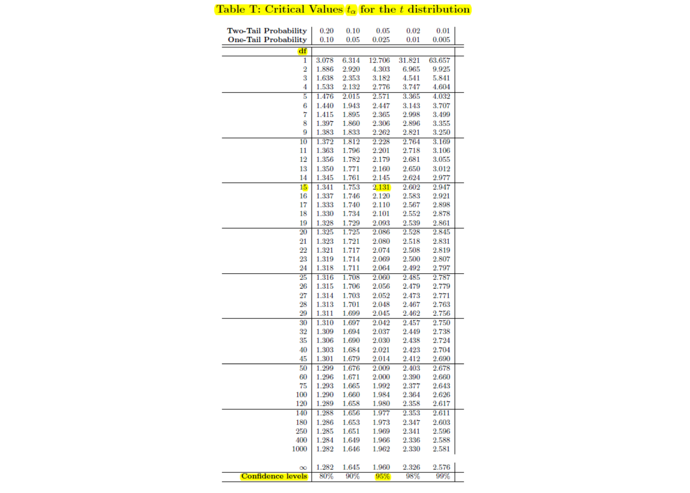
In our problem, we have the two-sided alternative hypothesis \(H_a: \mu_1 \neq \mu_2\), a test statistic \(t=2.261\), and \(df=28\).
We refer to the row for \(df=28\). Notice our test statistic \(t=2.261\) falls between the critical values \(t^*=2.048\) and \(t^*=2.467\).
Because we have a two-sided test, our \(p\)-value is \(.02<\text{p-value}<.05\).
Reject \(H_0\) at \(\alpha=.05\). We would have failed to reject \(H_0\) if we had used \(\alpha=0.01\).
Step Six: Conclusion
Since we rejected the null hypothesis, a proper conclusion would be:
The mean age of people in the treatment group is than the mean height of people in the control group.
Notice that the effect is said to be significantly different and NOT significantly greater. This is because we chose a two-sided alternative hypothesis rather than a one-sided hypothesis. This decision should be made a priori (before collecting data) and NOT changed just to get a ‘desired’ result.
20.2 Independent Samples \(t\)-test with Technology
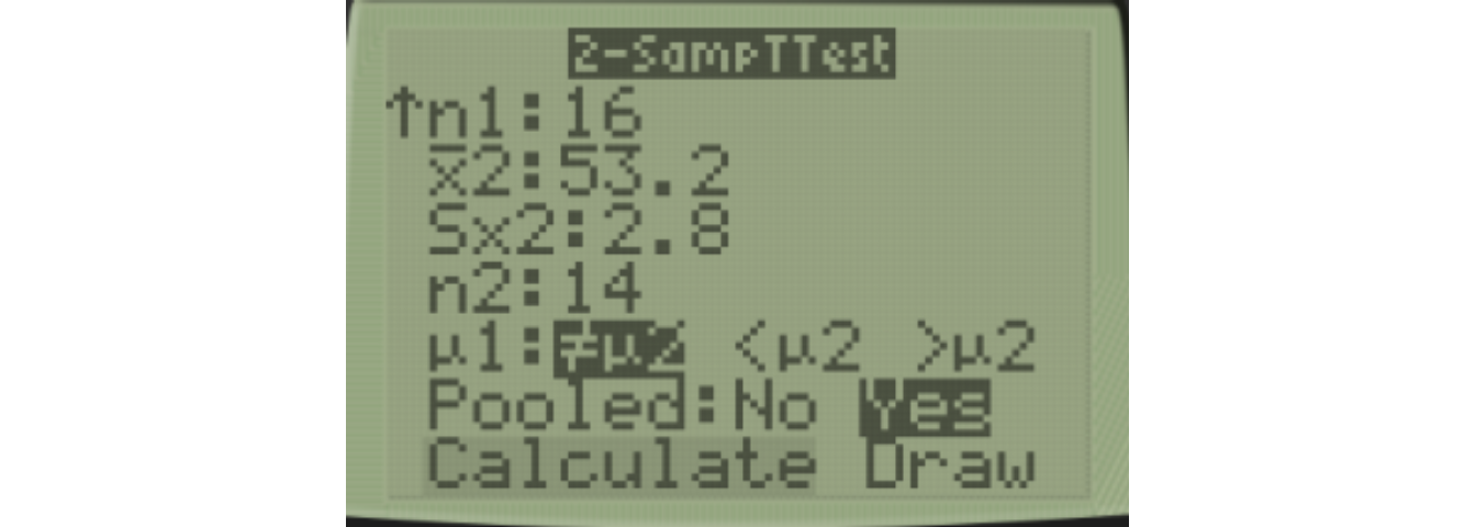
With a TI-83/84, go to STAT, then TESTS, and choose 4:2-SampTTest. You will use Inpt:Stats since we have the summary statistics but not the raw data, and Pooled=Yes since we use the pooled variance when assuming equal variances.

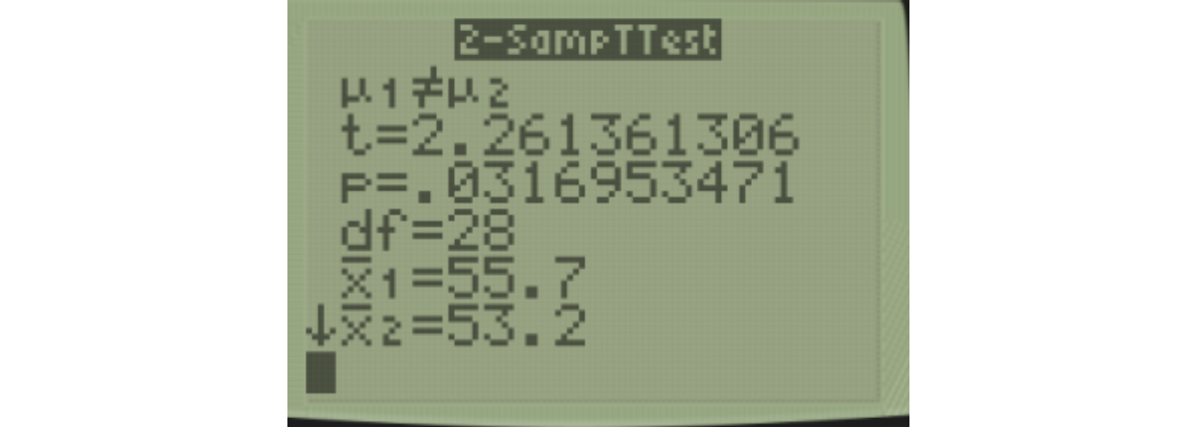
The results on our calculator agree with our earlier calculation.
20.3 Welch’s \(t\)-test for Unequal Variances
The assumption of equal variances is sometimes not met, and an alternative version of the \(t\)-test exists when we assume unequal variances. This test is often called Welch’s \(t'\)-test. This is shown in your book, although
\[t'=\frac{\bar{x_1}-\bar{x_2}}{\sqrt{\frac{s^2_1}{n_1}+\frac{s^2_2}{n_2}}}\]
Notice we do not need to compute \(s_p^2\), pooled variance. However, the degrees of freedom are no longer equal to \(n_1+n_2-2\). Instead, \(df\) is either computed by an ugly formula (details hidden), approximated with an easier formula, or approximated even further by treating it as a \(z\)-test (for large samples).
Let’s look at another example, this time assuming unequal variances.
Example: Suppose I am comparing final exam scores for two different sections of the same course, with one class having taken their final exams on Monday morning and the other on Friday afternoon. We wish to see if there is a significant difference in scores.
Step One: Write Hypotheses
\[H_0: \mu_F=\mu_M\] \[H_A: \mu_F \neq \mu_M\]
Step Two: Choose Level of Significance
Let \(\alpha=0.05\).
Step Three: Choose Test/Check Assumptions
I will choose the two-sample \(t\)-test. Assumptions include that the samples are independent, random, and normally distributed with unequal variances. Notice there is an outlier in the Friday class, but it is a real score and I will not change or drop the score.
## ________________________________
##   1 | 2: represents 12, leaf unit: 1
##     Monday$exam      Friday$exam
## ________________________________
##              |  2 |9
##              |  3 |
##             9|  4 |57
##             3|  5 |
##             3|  6 |23578
##        875111|  7 |24
##     987766311|  8 |027
##             7|  9 |36
##             0| 10 |
## ________________________________
## n:         20      15
## ________________________________
## class min Q1 median Q3 max mean sd n missing
## 1 F 29 62 68 82 96 68.66667 18.35626 15 0
## 2 M 49 71 81 87 100 78.65000 13.05565 20 0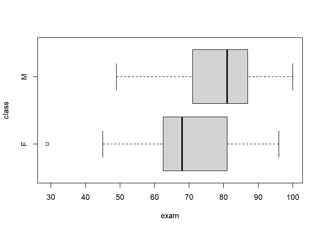
Step 4: Compute the test statistic
\[t'=\frac{\bar{x_1}-\bar{x_2}}{\sqrt{\frac{s^2_1}{n_1}+\frac{s^2_2}{n_2}}}\]
\[t'=\frac{68.66667-78.65}{\sqrt{\frac{18.35626^2}{15}+\frac{13.05565^2}{20}}}\]
\[t'=-1.793\]
Instead of using the complicated formula for degrees of freedom, I will use an approximation that will underestimate the df and thus provide a statistically conservative test that keeps \(\alpha\) below the stated level of 0.05.
\[df \approx min(n_1-1,n_2-1) \approx min(14,19) \approx 14\]
Step 5: Find p-value, Make Decision
In our problem, we have the two-sided alternative hypothesis \(H_a: \mu_1 \neq \mu_2\), a test statistic \(t`=-1.793\), and \(df \approx 14\).
We refer to the row for \(df=14\). Notice the absolute value of our test statistic \(|t'|=1.793\) falls between the critical values \(t^*=1.761\) and \(t^*=2.145\).
Because we have a two-sided test, our \(p\)-value is \(.05<\text{p-value}<.10\).
Fail to reject \(H_0\) at \(\alpha=.05\). (What would it have been if I had made a one-sided hypothesis that scores were lower on Friday?)
Step 6: Make Conclusion The means of the final exam scores are not statistically different between Monday and Friday.
Here’s what the results look like when I used software. Notice the exact \(df\) and \(p\)-value is computed by software so that an approximation for \(df\) and a table are not needed. This result is more accurate. The software also computes a 95% confidence interval for the difference in the two means.
If you decided to NOT use a \(t\)-test based on the outlier, I’ve also included results from the Mann-Whitney test (called the Wilcoxon Rank Sum Test by my software), a non-parametric alternative (we will not cover its formula).
##
##  Welch Two Sample t-test
##
## data:  exam by class
## t = -1.7935, df = 24.084, p-value = 0.08547
## alternative hypothesis: true difference in means between group F and group M is not equal to 0
## 95 percent confidence interval:
##  -21.469922   1.503255
## sample estimates:
## mean in group F mean in group M
##        68.66667        78.65000
##
## Wilcoxon rank sum test with continuity correction
##
## data: exam by class
## W = 96.5, p-value = 0.07706
## alternative hypothesis: true location shift is not equal to 020.4 Welch’s \(t\)-test with Technology
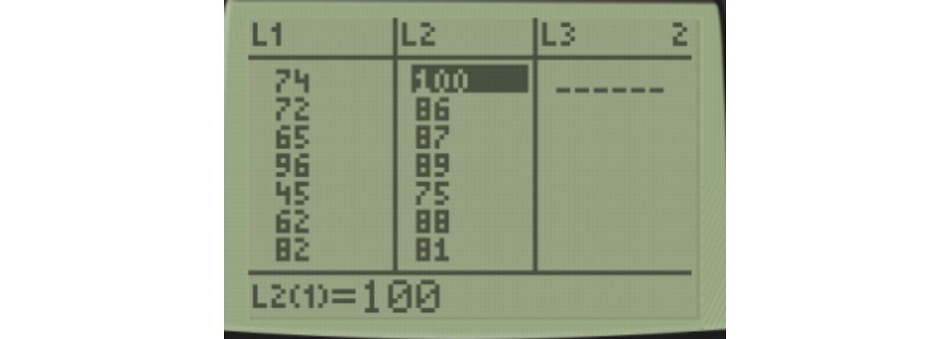
To do this problem with technology, I will manually enter the raw data into Lists L1 and L2.
\[\text{List 1 (Friday):} \: \: 74 \: 72 \: 65 \: 96 \: 45 \: 62 \: 82 \: 67 \: 63 \: 93 \: 29 \: 68 \: 47 \: 80 \: 87\]
\[\text{List 2 (Monday):} \: \: 100 \: 86 \: 87 \: 89 \: 75 \: 88 \: 81 \: 71 \: 87 \: 97 \: 83 \: 81 \: 49 \: 71 \: 63 \: 53 \: 77 \: 71 \: 86 \: 78\]
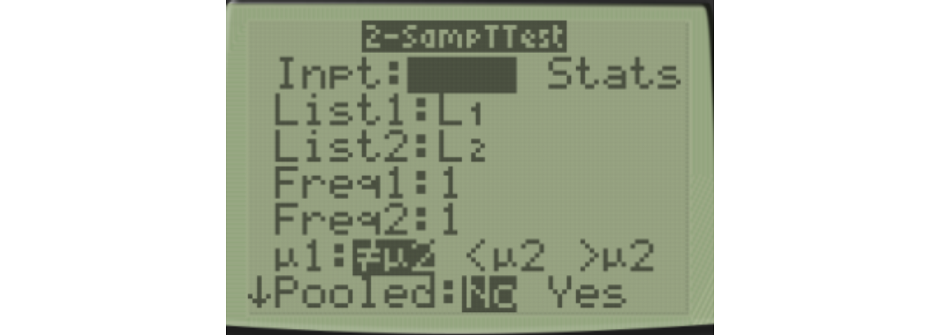
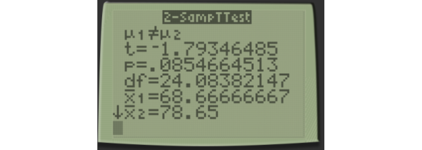
Notice that we do not have to use the conservative degrees of freedom, but can use the exact degrees of freedom calculated with an awful formula.
\[t=-1.793, df=24.084, p=0.0855\]
We fail to reject the null hypothesis at \(\alpha=0.05\) and conclude that there is not a statistically significant difference in exam scores between the Friday and Monday classes.
20.5 Confidence Interval for Difference in Means
Inference can also be done with a confidence interval rather than a hypothesis test. If we want a confidence interval of the difference in means, which is the parameter \(\mu_1 - \mu_2\), we have the same issue with the variances as in the hypothesis test.
We can assume equal variance, use \(df=n_1+n_2-2\) and the pooled variance.
\[\bar{x_1} - \bar{x_2} \pm t^* \sqrt{s_p^2(\frac{1}{n_1}+\frac{1}{n_2})}\]
Most modern textbooks recommend assuming unequal variances, and instead computing the confidence interval based on not using the pooled variance (i.e. similar to Welch’s \(t\)-test).
\[\bar{x_1} - \bar{x_2} \pm t^* \sqrt{\frac{s^2_1}{n_1}+\frac{s^2_2}{n_2}}\]
To obtain the critical value \(t^*\), one could use the conservative degrees of freedom \(df \approx \min(n_1-1,n_2-1)\). This will result in using a critical value larger than you should, and thus the margin of error of the interval would be too large.
It is preferable to use technology with the exact \(df\), which can be done on a TI calculator. Go to STAT, then TESTS, and choose 0:2-SampTInt.
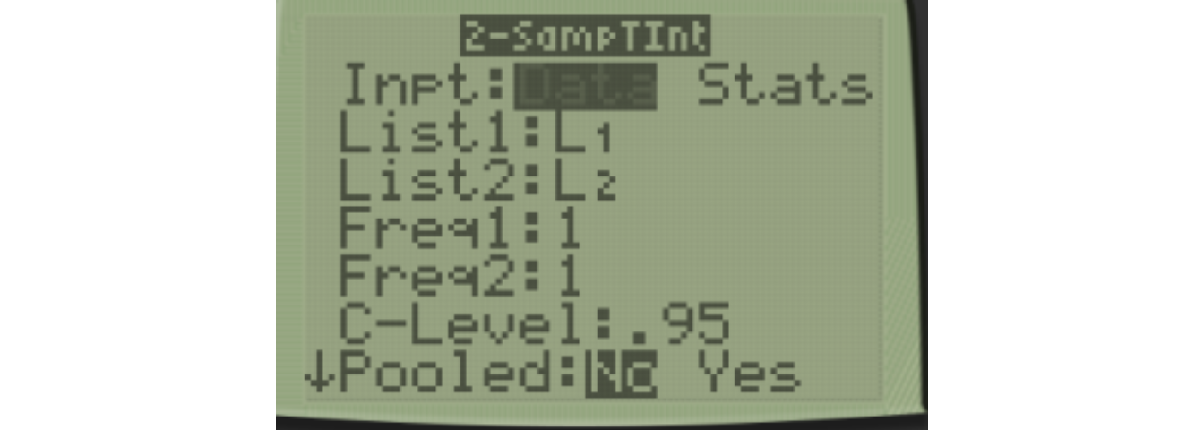
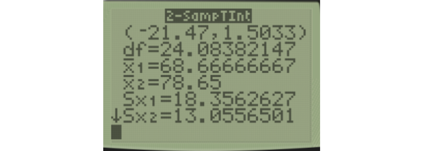
The 95% confidence interval for the difference of means, \(\mu_1-\mu_2\) is \[(-21.47,1.50)\]
Since this interval includes 0, this agrees with the decision to not reject the null hypothesis at the \(\alpha=0.05\) level.
The margin of error is half the width of the interval.
\[\text{Width} = \text{Upper} - \text{Lower}\]
\[\text{Width} = 1.50 - (-21.47) = 22.97\]
\[\text{Margin of Error} = \frac{1}{2}\text{Width}\]
\[\text{Margin of Error} = \frac{1}{2}(22.97) = 11.485\]
We could also report the confidence interval in the statistic plus/minus margin of error format:
\[\text{Statistic} \pm \text{Margin of Error}\]
\[ (\bar{x_1} - \bar{x_2}) \pm \text{Margin of Error}\]
\[ (68.667 - 78.65) \pm 11.485\]
\[ -9.983 \pm 11.485\]
The margin of error is larger than the absolute value of the statistic, so the difference is not statistically significant.