Chapter 12 Introduction to Probability
This roughly corresponds to chapters 12 and 13 of your textbook.
12.1 Definitions
Probability is the branch of mathematics that is concerned with assigned the likelihood of the occurrence of an event.
We often use formal and informal assessments of probability in everyday life. For example, you may check the weather before going to work to see the chance of rain, as predicted by meteorologists. Alternatively, you might just look out the window and determine for yourself if rain is likely or unlikely.
experiment: Broadly defined as any activity that we can observed where the result is a random event.
12.2 Outcomes and Events
outcome: one out of the many potential results of a random process (Examples: It rains tomorrow; I flip a coin and get ‘heads’; I roll two dice and get a total of 7; I ask a student what year of school they are in and they say ‘Freshman’)
event: A set of one or more of these outcomes. Typically denoted with letters at the beginning of the alphabet.
examples: \(A=\{heads\}\), \(B=\{7,11\}\), \(C=\{all \: freshaman \: and \: sophomores \}\)
12.3 Probability
The probability of an event is the relative likelihood of an event, which is \(0 \leq A \leq 1\). For \(P(A)=0\), the event must be impossible (i.e. the sum of 2 dice is equal to 1). For \(P(A)=1\), the event must be sure to happen (i.e. the sum of 2 dice is an integer). Values close to zero indicate an event unlikely to happen, while probabilities close to one indicate an event that is likely to happen.
We will spend a fair amount of time discussing how these probabilities are assigned.
12.4 Personal (Subjective) Probability
There are several methods for assigning the numerical values to the probability of an event occurring. If the event is based upon an experiment that cannot be repeated, we use the personal or subjective approach to probability.
Suppose I define event \(A\) to be the likelihood that it will rain today and I wish to know \(P(A)\). How can this be determined? Well, we could do a variety of things:
Look back on data from previous years on how often it rains on this date
Consult a weatherman (i.e. find the forecast on TV, radio, online)
Ask the old man who claims that if his knee aches, that means it is about to rain.
While some of these methods are more scientific than others (i.e. professional meteorologists have advanced climate models to use in assigning thes probabilities), this is based on an experiment which cannot be repeated, since we will observe and live through tomorrow only once. Maybe you remember the movie Groundhog Day or episodes of Star Trek: The Next Generation where the same day was repeated many times, but that doesn’t actually happen.
In class, I asked you to look up on your phone the ‘chance’ of rain in Murray today. Depending on where you looked it up, the percentage given was not always the same. Similarly, if I ask you what is the probability the St. Louis Cardinals win the World Series of baseball next year, I will get different answers. These answers depend on both one’s expertise and one’s bias (i.e. you might not follow baseball and have no idea or you might be a huge Cardinals fan and over-estimate the probability).
As an another example, we are interested in the probability that a patient who has just received a kidney transplant will survive for one year. This patient will only go through the next calendar year once, and will either survive or die. If the subjective probability is assigned by an expert, such as the patient’s surgeon, it might be fairly accurate.
However, subjective probability can be flawed if the probability is assigned by someone who is not an expert or is biased. If I am assigning the probability of the Chicago Cubs winning the World Series next year as \(P(C)=0.75\) (i.e. 75%), you could question both my baseball knowledge (or lack thereof) and my bias (I am a Cubs fan). For this reason, we try to avoid the subjective approach when possible.
12.5 Objective Probability
When we assign a numerical value to the probability of an event that CAN be repeated, we obtain an objective probability.
As the simplest type of experiment that can be repeated, consider flipping a coin, where event \(H\) is the probability of obtaining ‘heads’. I know you already know the answer to the question ‘What is \(P(H)\)?’, but suppose you are a Martian and have never encountered this strange object called a ‘coin’ before.
Our friendly Martian decides to conduct a simulation to determine \(P(H)\) by flipping the coin a large number of times. Suppose the Martian flips the coin 10,000 times and obtains 5,024 heads. His estimate of the probability is
\[ \begin{aligned} P(H) & = \frac{\text{number of occurrences of event}}{\text{total number of trials}} \\ P(H) & = \frac{5024}{10000} = 0.5024 \\ \end{aligned} \]
This is called the empirical or the relative frequency approach to probability. It is useful when the experiment can be simulated many, many times, especially when the mathematics for computing the exact probability is difficult or impossible.
12.6 Law of Large Numbers
The mathematician John Kerrich actually performed such an experiment when he was being held as a prisoner during World War II.
This example illustrates the Law of Large Numbers, where the relative frequency probability will get closer and closer to the true theoretical probability as the number of trials increase.
For instance, if I flipped a coin ten times and got 7 heads, you wouldn’t think anything was unusual, but if I flipped it 10,000 times and got heads 7,000 times, you would question the assumption that the coin was “fair” and the outcomes (heads or tails) were equally likely.
12.7 Classical Probability
The other type of objective probability is called classical probability, where we use mathematics to compute the exact probability without actually performing the experiment.
For example, we can determine \(P(H)\) without ever flipping a coin. We know there are two possible outcomes (heads and tails). If we are willing to assume the probability of each outcome is equally likely (i.e. a “fair” coin), then \(P(H)=\frac{1}{2}\).
Similarly, if we roll a single 6-sided die and let event \(A\) be the event that the die is less than 5, then notice that 4 of the 6 equally likely events contain our desired outcome, so \(P(A)=\frac{4}{6}\).
Clever mathematics, which can get quite difficult, can be used to compute probabilities of events such as the probability of getting a certain type of hand in a poker game or winning the jackpot in a lottery game such as Powerball.
12.8 Probabilities in Card Games
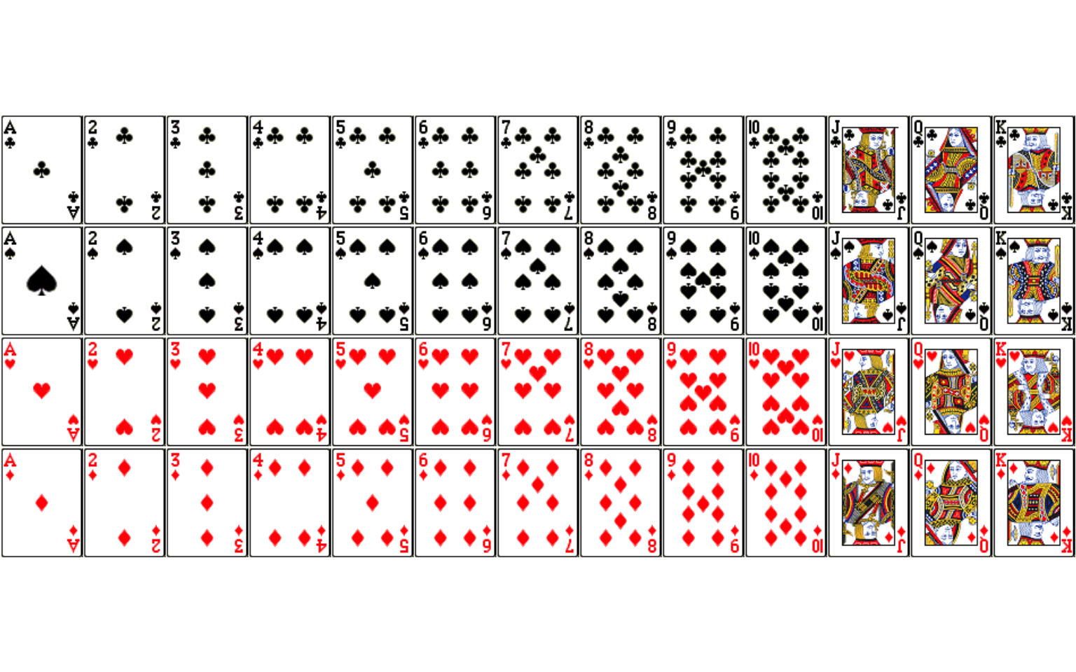
A standard deck of cards contains 52 cards. The cards are divided into 4 suits (spades, hearts, diamonds, clubs), where the spades and clubs are traditionally black and the hearts and diamonds are red. The deck is also divided into 13 ranks (2, 3, 4, 5, 6, 7, 8, 9, 10, Jack, Queen, King, Ace). The Jack, Queen, King are traditionally called face cards. The Ace can count as the highest and/or lowest ranking card, depending on the particular card game being played.
A player receives one card, at random, from the deck. Let \(A\) be the event the card is an Ace, \(B\) that the card is a heart, and \(C\) that the card is a face card.
\[P(A)=\frac{4}{52}=\frac{1}{13}\]
\[P(B)=\frac{13}{52}=\frac{1}{4}\]
\[P(C)=\frac{4+4+4}{52}=\frac{12}{52}\]
\[P(A \: and \: B)=\frac{4}{52}+\frac{13}{52}-\frac{1}{52}=\frac{16}{52}\]
\[P(A \: and \: C)=\frac{0}{52}=0\]
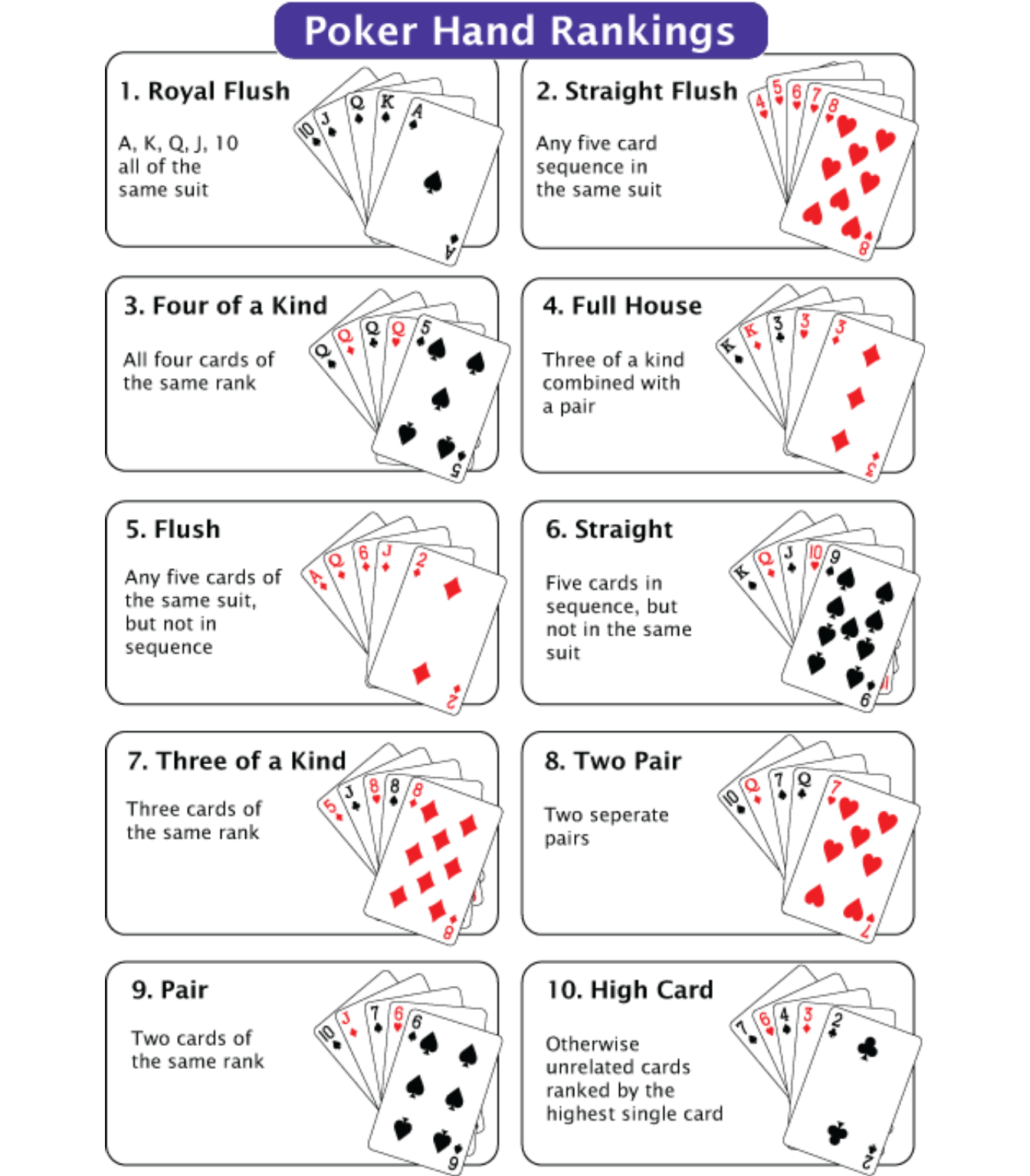
The popular card game poker can be played in many ways–the variation known as “Texas holdem” is currently the most popular. Most poker variations are based on ranking ones best 5 card hand, where the hand that is the hardest to get (i.e. has the lowest probability of occuring) is the winner.
A graph of the hands, from the strongest (royal flush, almost impossible to get), to the weakest (high card) is on the next page. Notice a “flush” (all cards same suit) beats a “straight”” (all cards in sequence or “order”) and that both of these hands beat a “three of a kind”.
12.9 Relative Frequency Approach to Poker
In class, we played three-card poker and empirically counted the probability of various hands happening. Should a flush still beat a straight? Is a three-of-a-kind easier or harder to get in three-card poker than the traditional five-card poker?
The results of our experiment with empirically counting the three-card poker hands (i.e. we perfored the experiment many times and counted how often certain outcomes occured)/
| Hand | Empirical Probability | Theoretical Probability |
|---|---|---|
| Straight Flush | \(\frac{8}{638}=.0125\) | .0022 |
| Flush | \(\frac{22}{638}=.0345\) | .0496 |
| Straight | \(\frac{22}{638}=.0345\) | .0326 |
| Three of a Kind | \(\frac{2}{638}=.0031\) | .0024 |
| One Pair | \(\frac{113}{638}=.1771\) | .1694 |
| High Card | \(\frac{471}{638}=.7382\) | .7489 |
We can clearly see (agreeing with intuition) that a three-of-a-kind is much harder to get in 3-card poker than 5-card poker, and should beat boths straights and flushes. In fact, the three-of-a-kind is almost as hard to get as a straight flush!
We would need a larger sample size (i.e. more trials of the experiment) to empirically determine that a straight is harder to get than a flush in 3-card poker, and thus the hand rankings should change.
12.10 Classical Probability, Poker
The mathematical notation for combinations, i.e. how many arrangements of \(r\) objects can be chosen from \(n\) objects, where order does not matter, is \[{ n \choose r}=\frac{n!}{r!(n-r)!}\]
For example \({52 \choose 2}\) would count the number of combinations if you were dealt 2 cards from a deck of 52. A Texas holdem poker player would be interested in this, as this game starts with each player being dealt 2 cards face down.
\[{52 \choose 2}=\frac{52!}{2! \times 50!}=\frac{52 \times 51 \times 50!}{2 \times 50!}=\frac{52 \times 51}{2}=1326\]
Notice that \({52 \choose 3}=22,100\) while \({52 \choose 5}=2,598,960\). The number of possible poker hands increases rapidly as more cards are added to the hand.
12.11 Classical Probability, Three-Card Poker
Here, I will find the probability of three-of-a-kind and one pair, when dealt three cards.
\[ \begin{aligned} P(Three-of-a-kind) & = & \frac{{13 \choose 1}{4 \choose 3}}{{52 \choose 3}} \\ & = & \frac{13 \times 4}{22100} \\ & = & \frac{52}{22100} \\ & = & .0024 \\ \end{aligned} \]
\[ \begin{aligned} P(One \: Pair) & = & \frac{{13 \choose 1}{4 \choose 2}{12 \choose 1}{4 \choose 1}}{{52 \choose 3}} \\ & = & \frac{13 \times 6 \times 12 \times 4}{22100} \\ & = & \frac{3744}{22100} \\ & = & .1694 \\ \end{aligned} \]
Finding the probabilities of certain other types of hands, such as straight, flushes, and straight flushes, is more complicated. Below I find the probability of getting three cards, all the same suit, but this includes both regular flushes and straight flushes. We will not pursue these probabilities in more detail; the interested student can go to http://people.math.sfu.ca/~alspach/computations.html for detailed computations of many poker scenarios.
\[ \begin{aligned} P(Same \: Suit) & = & \frac{{4 \choose 1}{13 \choose 3}}{{52 \choose 3}} \\ & = & \frac{4 \times 286}{22100} \\ & = & \frac{1144}{22100} \\ \end{aligned} \]
12.12 Blood Type Problem
Suppose everyone in the population has one and exactly one of the four basic blood types (O, A, B, and AB). This is roughly true. Notice, we are not considering the Rh factor \(+\) or \(-\) in this problem.
The percentages in the table below are roughly true for the US population. These probabilities will fluctuate for different countries, as certain blood types are more or less common among certain ethnic groups.
| Blood Type | Probability |
|---|---|
| Type O | 0.45 |
| Type A | 0.40 |
| Type B | 0.11 |
| Type AB | ? |
Suppose I choose one person at random:
\(P(AB)=1-(.45+.40+.11)=1-.96=.04\) or about 4% have Type AB blood.
\(P(A \: or :\ B) = .40 + .11 = .51\) or about 51% have either Type A or Type B blood. This is a specific application of the Addition Rule where we assume that the two events are disjoint (i.e. no one person has both Type A and Type B blood)
\(P(not :\ O)=P(O^c)=1-P(O)=1-.45=.55\), or about 55% do not have Type O blood. This is called the Complement Rule, which finds the probability of some event not occuring. There are sitautions where finding the probability of the “complement”, such as \(P(not :\ 0)\), also called \(P(O^c)\) is much easier than the probability of the event itself, \(P(O)\).
Suppose I choose two people at random, in such a way as the people are independent (i.e. the probability of events do not depend on each other).
\(P(both \: have \: Type \: A) = .40 \times .40 = .16\)
Some harder probabilities:
\(P(all \: 3 \: are \: Type \: O) = .45 \times .45 \times .45 = (.45)^3\)
\(P(none \: have \: Type \: AB) = (1-.04)^3 = (.96)^3\)
\(P(at \: least \: one \: is \: Type \: B) = ???\)
The last problem is easier if we find the probability of the complement (the opposite is the probability that none have Type B), and subtract that probability from one.
\(P(at \: least \: one \: is \: Type \: B) = 1 - (1-.11)^3 = 1-(.89)^3\)
12.13 Let’s Make a Deal (Monte Hall problem)
This is a pretty well-known problem, based on the game show Let’s Make a Deal. It is sometimes called the Monte Hall problem, after the host of the show back in the 1960s and 1970s.
There are three doors; behind one is a prize (say a car or lots of money which you want), and behind the other two is no prize (or something you don’t want). You choose a door, and the game show host shows you one of the doors you didn’t choose, where there is no prize. The host (Monte Hall or Wayne Brady) offers you a chance to switch to the other unopened door.
Should you switch doors?
Should you stay with your first choice?
Maybe it doesn’t matter and you could just flip a coin…
If you saw the TV show ‘Numb3rs’ or the movie ‘Twenty-One’, the problem was featured: http://youtu.be/OBpEFqjkPO8
You can simulate the game here: http://www.rossmanchance.com/applets/MontyHall/Monty04.html
Why is it better for you to switch your choice than stay with your initial guess? (You might draw a tree diagram to see why)