Chapter 16 Confidence Intervals for Proportions
16.1 Binomial Distribution with large \(n\)
What happens to the shape of the binomial distribution as \(n\) gets large? Here’s the picture of our binomial example
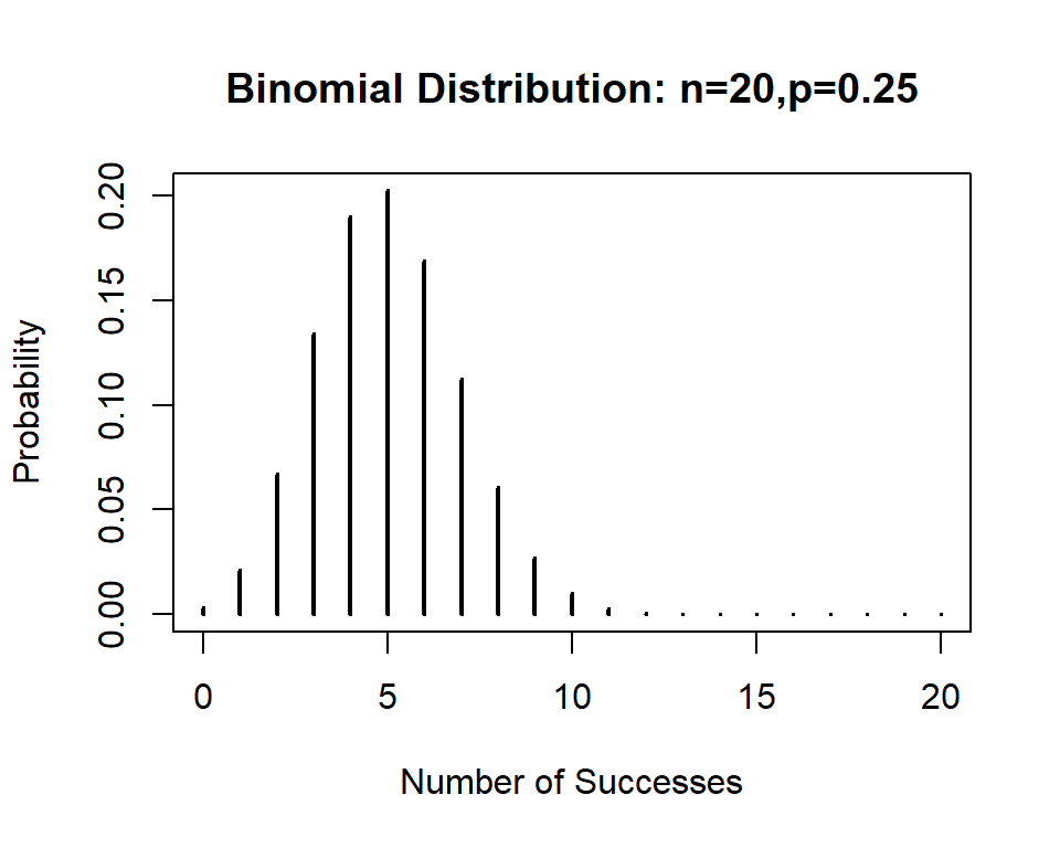
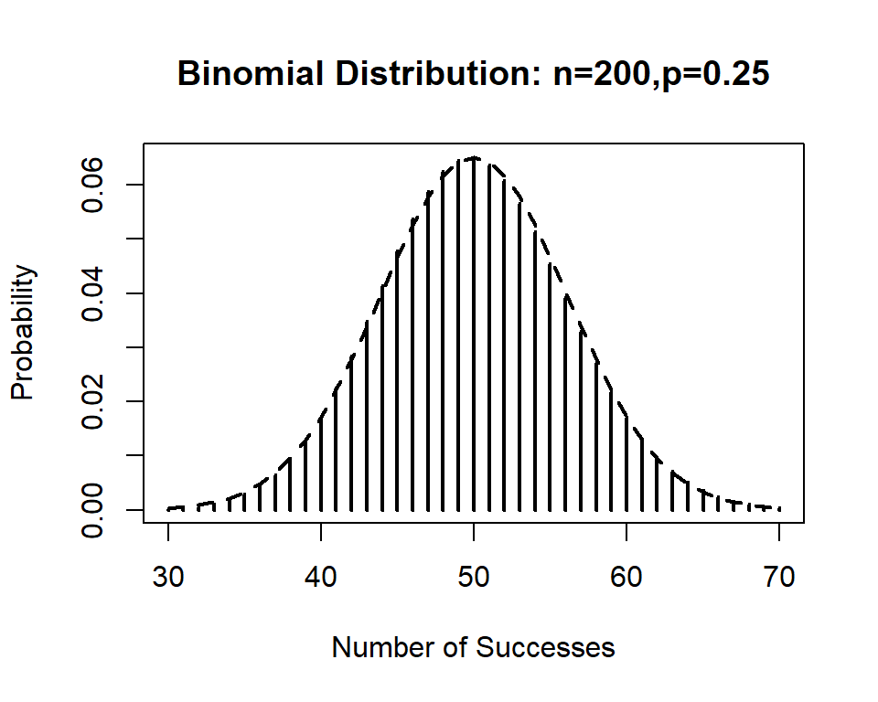
This is right skewed. Now I will increase \(n=200\); notice the new graph is almost perfectly symmetric and is similar to the normal distribution. The dotted line is a normal distribution with the same mean and standard deviation as the binomial; \(\mu=200(.25)=50\), \(\sigma=\sqrt{200(.25)(.75)}=\sqrt{37.5}\)
16.2 Normal Approximation to the Binomial
What if we try to use the binomial distribution for a very large value of \(n\)? The binomial distribution (which is discrete) can be well approximated by the normal distribution (which is continuous) when:
\(np \geq 10\) (expected number of successes)
\(n(1-p)= nq \geq 10\) (expected number of failures)
If \(X \sim BIN(n,p)\) with \(n\) large enough as given above, then
\[X \dot{\sim} N(\mu=np, \sigma=\sqrt{npq})\]
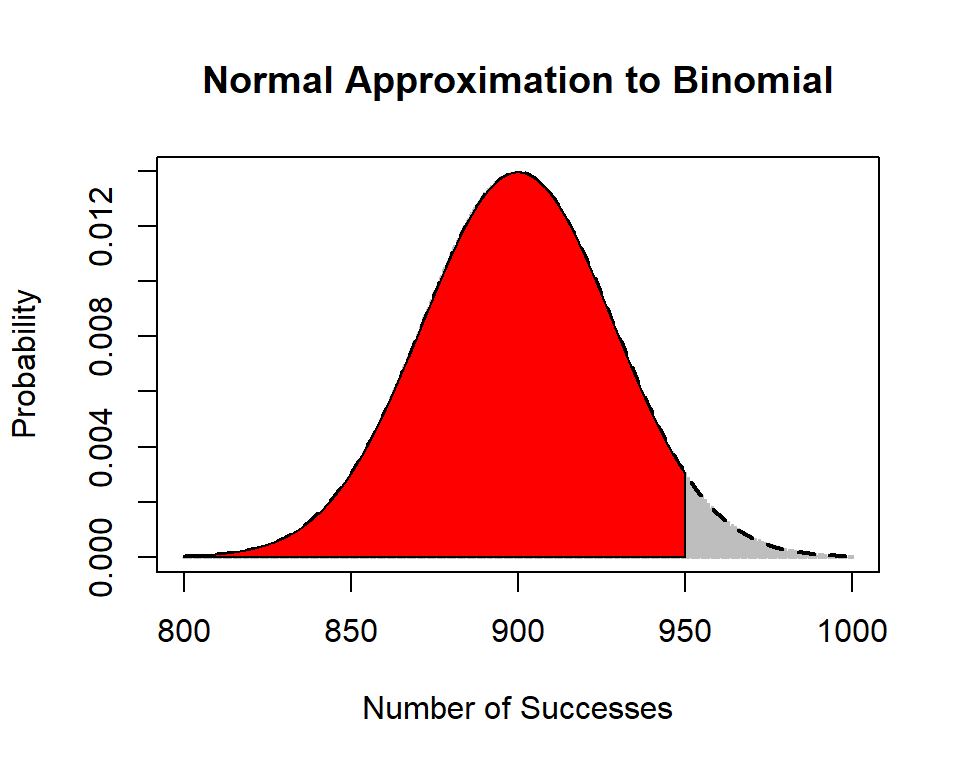
Example: Suppose in a sample of \(n=10000\) people, 9% have the flu. Notice that \(\mu=10000(.09)=900\) and \(\sigma=\sqrt{10000(.09)(.91)}=\sqrt{819}\).
I want to find \(P(X \leq 950)\) with the normal approximation.
First, check the number of expected successes and failures. \(np=10000(0.09)=900\), \(nq=10000(.91)=9100\). Both are much larger than 10. So \(X \dot{\sim} N(\mu=900, \sigma=\sqrt{819})\).
I will turn \(X=950\) into a \(z\)-score.
\(Z=\frac{X-\mu}{\sigma}=\frac{950-900}{\sqrt{819}}=1.75\).
\(P(X \leq 950)=P(Z \leq 1.75)=0.9599\) (table)
or \(P(X \leq 950)=\) normalcdf(-1E99,950,900,sqrt(819)) = .9597.
16.3 Sampling Distributions
What is a sampling distribution?
We will take a random sample of size \(n\)
We will calculate some statistic based on our random sample. It might be the sample mean \(\bar{x}\) or the sample proportion \(\hat{p}\), where \[\hat{p}=\frac{x}{n}=\frac{successes}{trials}\]
Imagine that we collected a very large number of random samples, and we calculated that statistic for each and every random sample.
The sampling distribution is the distribution that consists of all of the statistics computed from each sample.
Examples:
- Suppose we flipped a coin \(n=20\) times a day, computed \(\hat{p}\) each day, and graphed all of our \(\hat{p}\) in a histogram. In this case, it seems like the mean of all of our \(\hat{p}\)s should be equal to the parameter’s true value \(p=0.50\). (What does that histogram remind you of?)
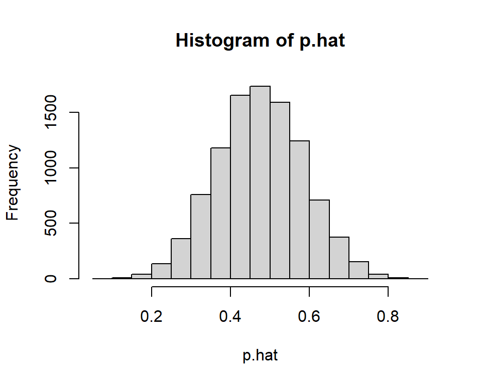
## [1] 0.50037## [1] 0.1113266What if we flipped the coin \(n=100\) times a day instead? What do you notice is different about the sampling distribution when the sample size \(n\) is increased?
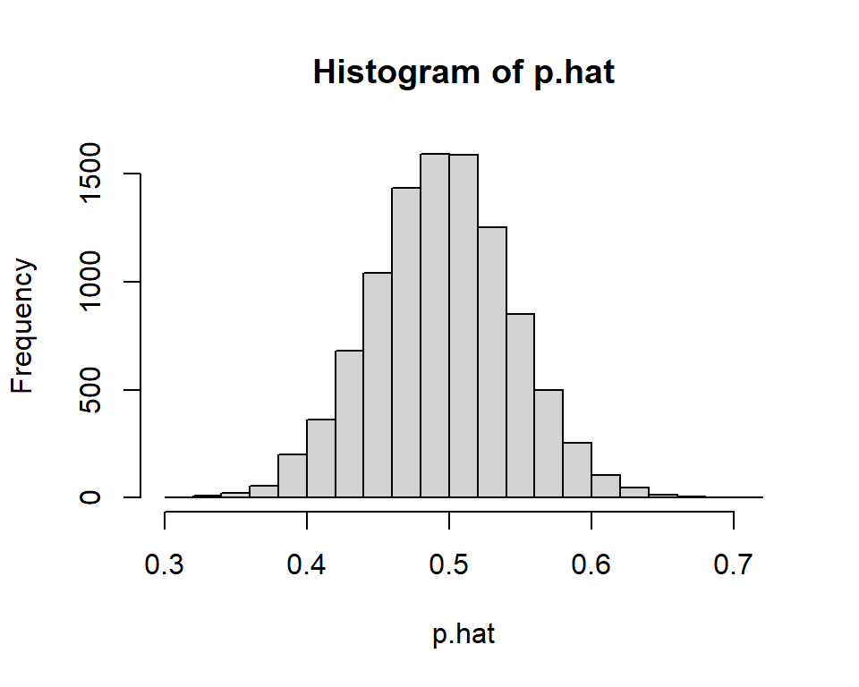
## [1] 0.499889## [1] 0.04944332For proportions, the mean of the sampling distribution is: \[\mu_{\hat{p}}=p\]
The standard deviation of the sampling distribution (called the standard error) is: \[\sigma_{\hat{p}}=\sqrt{\frac{p(1-p)}{n}}\]
16.4 Confidence Interval of the Sample Proportion
If the sample is ‘large’ enough with both \(np\) and \(nq\) 10 or more, then \(\hat{p}\) will be approximately normal.
\[\hat{p} \dot{\sim} N(p,\sqrt{\frac{p(1-p)}{n}})\]
This is the basis for our formula for the confidence interval for \(p\) in chapter 16 and will also be used when we study hypothesis testing for a proportion later on.
\[\hat{p} \pm z^* \sqrt{\frac{\hat{p}(1-\hat{p})}{n}}\]
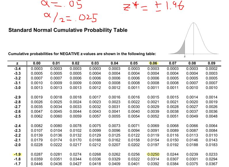
Values of \(z^*\) are \(\pm 1.96\) for 95% confidence (\(\alpha=0.05\)), \(\pm 2.576\) for 99% confidence (\(\alpha=0.01\)), and \(\pm 1.645\) for 90% confidence (\(\alpha=0.10\)).
ZTableCriticalValue
You could also determine these \(z^*\) critical values by using invNorm(0.025), invNorm(0.975), or in general use \(\alpha/2\) and \(1-\alpha/2\).
On the calculator, go to STAT, TESTS, A:1-PropZInterval.
The right-hand side of the formula is the margin of error, which is found by multiplying the critical value (in this case, a \(z\)-score from the normal distribution) times the standard error of the proportion.
Soon, we will see that if \(X \sim N(\mu,\sigma)\), then \(\bar{X} \sim N(\mu, \sigma/\sqrt{n})\) and a similar formula can be used for the confidence interval for \(\mu\), if \(\sigma\) is known. Later, we’ll cover the more realistic situation when \(\sigma\) is not known.
On the calculator, go to STAT, TESTS, 7:ZInterval.
\[\bar{x} \pm z^* \frac{\sigma}{\sqrt{n}}\]
16.5 Gallup Poll example
Here is a (somewhat) recent poll taken by the Gallup organizaion, regarding U.S. households that has been victimized by crime.
http://www.gallup.com/poll/179174/one-four-households-victimized-crime.aspx
PRINCETON, N.J. – Twenty-six percent of Americans say they or another member of their household were the victim of some type of property or physical crime in the last 12 months, ranging from theft to sexual assault, according to Gallup’s index of crime victimization. Since 2000, the percentage of households that have been victimized by crime has ranged narrowly between 22% and 27%. The percentage of Americans who have been personally victimized has ranged from 14% to 19%.

graph
Survey Methods
Results for this Gallup poll are based on telephone interviews conducted Oct. 12-15, 2014, with a random sample of 1,017 adults, aged 18 and older, living in all 50 U.S. states and the District of Columbia.
For results based on the total sample of national adults, the margin of sampling error is \(\pm 4\) percentage points at the 95% confidence level.
Each sample of national adults includes a minimum quota of 50% cellphone respondents and 50% landline respondents, with additional minimum quotas by time zone within region. Landline and cellular telephone numbers are selected using random-digit-dial methods.
It is important to realize that the \(\pm 4\)% that the Gallup organization reports was NOT computed with the formula that we use in class. Our formula assumes a simple random sample. For stratified samples, cluster samples, and complex multistage samples that these companies use, other formulas are needed; essentially, the standard error part of the formula becomes more complex. The simpler formula for margin of error that we will cover is a good approximation for the results that the professional pollsters will get.
16.6 Correct and Incorrect Interpretations of a CI
Suppose we have taken a random sample (i.i.d. or simple) of \(n=500\) voters, where \(X=220\) support Richard Guy, a candidate for political office. The point estimate is \[\hat{\pi}=\frac{220}{500}=0.44\]
The interval estimate for 95% confidence is \[ \begin{aligned} \hat{\pi} & \pm z^* \sqrt{\frac{\hat{\pi}(1-\hat{\pi})}{n}} \\ 0.44 & \pm 1.96 \sqrt{\frac{0.44(1-0.44)}{500}} \\ 0.44 & \pm 0.0435 \\ & (0.3965,0.4835) \\ \end{aligned} \]
The margin of error of our poll is \(\pm 4.35\)% and the entire intervals lies below \(\pi=0.50\), which is bad news for Richard Guy in his election.
What will happen to the margin of error if the sample size increases? If we double the sample size, will we cut the margin of error in half?
What will happen to the margin of error if we increase the confidence level from the usual 95% level to the 99% level?
NOTE: This does NOT mean that there is a 95% chance that the true value of \(\pi\) is between 0.3965 and 0.4835. It means that we are 95% confident that our random sample ‘captured’ the true value of \(\pi\).
We realize that 95% of CIs drawn from random samples of our size will capture the true value of \(p\) and 5% are ‘unlucky’ and miss the true value of \(p\).
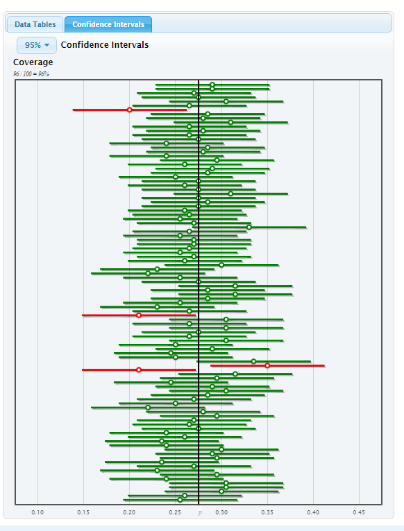
A nifty applet for showing this visually can be obtained in StatKey. Go to the l StatKey page http://lock5stat.com/statkey/index.html and click on Sampling Distributions: Proportion (right hand side). We’ll use their College Graduates example. This example is based on the fact that 27.5% of Americans are college graduates; in other words, we know that the parameter \(p=0.275\). Click on the Confidence Intervals tab on the right and Generate 100 Samples. Each of the bootstrap samples has a CI that is graphed; ones that included the true parameter \(p=0.275\) show up in green; ones that miss show up in red. Over the long run, about 5% should miss, so we expect about 5 red CIs. I got 96 green CIs and 4 red CIs that ‘missed’ when I took 100 random samples of size \(n=200\) from this population.
CIs