Exercise 9 EFA of polytomous item scores
| Data file | CHI_ESQ.txt |
| R package | psych |
9.1 Objectives
The objective of this exercise is to conduct Exploratory Factor Analysis (EFA) of polytomous responses to a short service satisfaction questionnaire. Despite the aim of this questionnaire to measure one construct, user satisfaction, the analysis will reveal that more than one factor is responsible for the items’ co-variation.
9.2 Study of service satisfaction using Experience of Service Questionnaire (CHI-ESQ)
In 2002, Commission for Health Improvement in the UK developed the Experience of Service Questionnaire (CHI-ESQ) to measure user experiences with the Child and Adolescent Mental Health Services (CAMHS). The questionnaire exists in two versions: one for older children and adolescents for describing experiences with their own treatment, and the other is for parents/carers of children who underwent treatment. We will consider the version for parents/carers.
The CHI-ESQ parent version consists of 12 questions covering different types of experiences. Here are the questions:
1. I feel that the people who have seen my child listened to me
2. It was easy to talk to the people who have seen my child
3. I was treated well by the people who have seen my child
4. My views and worries were taken seriously
5. I feel the people here know how to help with the problem I came for
6. I have been given enough explanation about the help available here
7. I feel that the people who have seen my child are working together to help with the problem(s)
8. The facilities here are comfortable (e.g. waiting area)
9. The appointments are usually at a convenient time (e.g. don’t interfere with work, school)
10. It is quite easy to get to the place where the appointments are
11. If a friend needed similar help, I would recommend that he or she come here
12. Overall, the help I have received here is good
Parents/carers are asked to respond to these questions using response options “Certainly True” — “Partly True” — “Not True” (coded 1-2-3) and Don’t know (not scored but treated as missing data, “NA”).
Participants in this study are N=620 parents reporting on experiences with one CAMHS member Service. This is a subset of the large multi-service sample analysed and reported in Brown, Ford, Deighton, & Wolpert (2014).
9.3 Worked Example - EFA of responses to CHI-ESQ parental version
To complete this exercise, you need to repeat the analysis from a worked example below, and answer some questions.
Step 1. Reading and examining the data
I recommend you download data file CHI_ESQ.txt into a new folder, and in RStudio, associate a new project with this folder. Create a new script, where you will type all commands.
The data are stored in the space-separated (.txt) format. You can preview the file by clicking on CHI_ESQ.txt in the Files tab in RStudio (this will not import the data yet, just open the actual file). You will see that the first row contains the item abbreviations (esq+p for “parent”): “esqp_01”, “esqp_02”, “esqp_03”, etc., and the first entry in each row is the respondent number: “1”, “2”, …“620”. Function read.table() will import this into RStudio taking care of these column and row names. It will actually understand that we have headers and row names because the first row contains one fewer fields than the number of columns (see ?read.table for detailed help on this function).
We have just read the data into a new data frame named CHI_ESQ. Examine the data frame by either pressing on it in the Environment tab, or calling function View(CHI_ESQ). You will see that there are quite a few missing responses, which could have occurred because either “Don’t know” response option was chosen, or because the question was not answered at all.
Step 2. Examining suitability of data for factor analysis
First, load the package psych to enable access to its functionality. Conveniently, most functions in this package easily accommodate analysis with correlation matrices as well as with raw data.
Before we start EFA, it is always good to examine correlations between variables. Function lowerCor() from package psych provides these correlations in a convenient format.
##         es_01 es_02 es_03 es_04 es_05 es_06 es_07 es_08 es_09 es_10 es_11
## esqp_01 1.00
## esqp_02 0.67  1.00
## esqp_03 0.65  0.68  1.00
## esqp_04 0.79  0.65  0.67  1.00
## esqp_05 0.61  0.54  0.52  0.64  1.00
## esqp_06 0.58  0.55  0.50  0.60  0.68  1.00
## esqp_07 0.60  0.50  0.55  0.63  0.71  0.70  1.00
## esqp_08 0.15  0.25  0.21  0.22  0.14  0.30  0.21  1.00
## esqp_09 0.24  0.26  0.18  0.19  0.18  0.24  0.16  0.31  1.00
## esqp_10 0.17  0.25  0.19  0.15  0.14  0.18  0.15  0.36  0.28  1.00
## esqp_11 0.63  0.53  0.60  0.60  0.61  0.55  0.58  0.22  0.20  0.22  1.00
## esqp_12 0.72  0.60  0.62  0.72  0.71  0.66  0.68  0.22  0.21  0.15  0.71
## [1] 1.00
Examine the correlations carefully. Notice that all correlations are positive. However, there is a pattern to these correlations. While most are large (above 0.5), correlations between items esqp_08, esqp_09, esqp_10 (describing experiences with facilities, appointment times and location) and the rest of the items (describing experiences with treatment) are substantially lower, ranging between 0.14 and 0.30. Correlations of these items among each other are only slightly larger, ranging between 0.28 and 0.36. We will see whether and how EFA will pick up on this pattern of correlations.
Now, request the Kaiser-Meyer-Olkin (KMO) index – the measure of sampling adequacy (MSA):
## Kaiser-Meyer-Olkin factor adequacy
## Call: KMO(r = CHI_ESQ)
## Overall MSA =  0.92
## MSA for each item =
## esqp_01 esqp_02 esqp_03 esqp_04 esqp_05 esqp_06 esqp_07 esqp_08 esqp_09 esqp_10
##    0.92    0.93    0.93    0.92    0.93    0.93    0.93    0.76    0.86    0.80
## esqp_11 esqp_12
##    0.95    0.94
QUESTION 1. What is the overall measure of sampling adequacy (MSA)? Interpret this result.
Step 3. Determining the number of factors
We will use function fa.parallel() to produce a scree plot for the observed data, and compare it to that of a random (i.e. uncorrelated) data matrix of the same size. We will use the default estimation method (fm="minres"), because the data are responses with only 3 ordered categories, where we cannot expect a normal distribution. We will again display only eigenvalues for principal components (fa="pc"), as is done in commercial software packages such as Mplus.
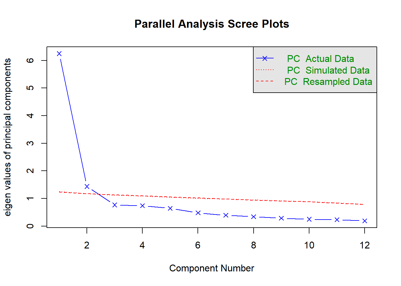
## Parallel analysis suggests that the number of factors = NA and the number of components = 2QUESTION 2. Examine the Scree plot. Does it support the hypothesis that 1 factor - satisfaction with service - underlie the data? Why? Does your conclusion correspond to the text output of the parallel analysis function?
Step 4. Fitting an exploratory 1-factor model and assessing the model fit
We will use function fa(), which has the following general form
fa(r, nfactors=1, n.obs = NA, rotate="oblimin", fm="minres" …),
and requires data (argument r), and the number of observations if the data is correlation matrix (n.obs). Other arguments have defaults, which we are happy with for the first analysis.
Specifying all necessary arguments, test the hypothesized 1-factor model:
# fit 1-factor model
fit1 <- fa(CHI_ESQ, nfactors=1)
# print short summary with model fit
summary.psych(fit1)
##
## Factor analysis with Call: fa(r = CHI_ESQ, nfactors = 1)
##
## Test of the hypothesis that 1 factor is sufficient.
## The degrees of freedom for the model is 54 and the objective function was 0.92
## The number of observations was 620 with Chi Square = 562.91 with prob < 7.7e-86
##
## The root mean square of the residuals (RMSA) is 0.07
## The df corrected root mean square of the residuals is 0.08
##
## Tucker Lewis Index of factoring reliability = 0.86
## RMSEA index = 0.123 and the 10 % confidence intervals are 0.114 0.133
## BIC = 215.7From the summary output, we find that Chi Square = 562.91 (df = 54) with prob < 7.7e-86 - a highly significant result. According to the chi-square test, we have to reject the model. We also find that the root mean square of the residuals (RMSR) is 0.07. According to the commonly used threshold of 0.08 for an acceptable fit, this model fits acceptably.
Next, let’s examine the model residuals, which are direct measures of model (mis)fit.
##         es_01 es_02 es_03 es_04 es_05 es_06 es_07 es_08 es_09 es_10 es_11
## esqp_01    NA
## esqp_02  0.05    NA
## esqp_03  0.03  0.12    NA
## esqp_04  0.10  0.03  0.04    NA
## esqp_05 -0.04 -0.05 -0.07 -0.02    NA
## esqp_06 -0.06 -0.02 -0.07 -0.04  0.08    NA
## esqp_07 -0.04 -0.08 -0.03 -0.03  0.10  0.11    NA
## esqp_08 -0.09  0.03 -0.01 -0.03 -0.09  0.08 -0.02    NA
## esqp_09  0.00  0.05 -0.03 -0.05 -0.04  0.03 -0.06  0.23    NA
## esqp_10 -0.03  0.06  0.01 -0.06 -0.05 -0.01 -0.04  0.28  0.21    NA
## esqp_11  0.00 -0.03  0.03 -0.04  0.01 -0.03 -0.01  0.00 -0.01  0.03    NA
## esqp_12  0.01 -0.05 -0.02  0.00  0.04  0.00  0.02 -0.03 -0.04 -0.07  0.06
## [1]    NA
You can see that the residuals are all small except one cluster corresponding to the correlations between items esqp_08, esqp_09, and esqp_10, where residuals are between 0.21 and 0.28. Evidently, one factor can explain the observed correlations between items 1-7 and 11-12, but it cannot fully explain the pattern of correlations we observed between items 8-10 (which describe experience with facilities, appointment times and location rather than treatment as the rest of items). Quite intuitively, one factor can explain the overall positive manifold of all correlations, but not a complex pattern we observe here.
We conclude that the 1-factor model is clearly not adequate for these data.
Step 5. Fitting an exploratory 2-factor model and assessing the model fit
Now let’s fit a 2-factor model to these data:
## Loading required namespace: GPArotation##
## Factor analysis with Call: fa(r = CHI_ESQ, nfactors = 2)
##
## Test of the hypothesis that 2 factors are sufficient.
## The degrees of freedom for the model is 43 and the objective function was 0.64
## The number of observations was 620 with Chi Square = 394 with prob < 3e-58
##
## The root mean square of the residuals (RMSA) is 0.04
## The df corrected root mean square of the residuals is 0.05
##
## Tucker Lewis Index of factoring reliability = 0.878
## RMSEA index = 0.115 and the 10 % confidence intervals are 0.105 0.125
## BIC = 117.52
## With factor correlations of
## MR1 MR2
## MR1 1.00 0.39
## MR2 0.39 1.00QUESTION 3. What is the chi square statistic, and p value, for the tested 2-factor model? Would you retain or reject this model based on the chi-square test? Why?
QUESTION 4. Find and interpret the RMSR in the output.
Examine the 2-factor model residuals.
##         es_01 es_02 es_03 es_04 es_05 es_06 es_07 es_08 es_09 es_10 es_11
## esqp_01    NA
## esqp_02  0.05    NA
## esqp_03  0.03  0.12    NA
## esqp_04  0.09  0.03  0.04    NA
## esqp_05 -0.05 -0.04 -0.07 -0.03    NA
## esqp_06 -0.06 -0.02 -0.07 -0.04  0.09    NA
## esqp_07 -0.05 -0.07 -0.03 -0.04  0.08  0.11    NA
## esqp_08 -0.05 -0.03 -0.02  0.02 -0.02  0.05  0.03    NA
## esqp_09  0.04  0.01 -0.03 -0.01  0.01  0.01 -0.02  0.00    NA
## esqp_10  0.01  0.01  0.01 -0.02  0.02 -0.03  0.00  0.00  0.00    NA
## esqp_11  0.00 -0.03  0.03 -0.04  0.01 -0.03 -0.01  0.00 -0.01  0.03    NA
## esqp_12 -0.01 -0.04 -0.02 -0.02  0.02  0.01  0.00  0.02  0.01 -0.02  0.06
## [1]    NA
QUESTION 5. Examine the residual correlations. What can you say about them? Are there any non-trivial residuals (greater than 0.1 in absolute value)?
Step 6. Interpreting the 2-factor un-rotated solution
Having largely confirmed suitability of the 2-factor model, are are ready to examine and interpret its results. We will start with an un-rotated solution.
##
## Loadings:
##         MR1    MR2
## esqp_01  0.829
## esqp_02  0.749
## esqp_03  0.748
## esqp_04  0.840 -0.104
## esqp_05  0.788 -0.155
## esqp_06  0.764
## esqp_07  0.777 -0.110
## esqp_08  0.310  0.551
## esqp_09  0.291  0.403
## esqp_10  0.259  0.501
## esqp_11  0.756
## esqp_12  0.859 -0.121
##
##                 MR1   MR2
## SS loadings    5.88 0.797
## Proportion Var 0.49 0.066
## Cumulative Var 0.49 0.556
The un-rotated solution yields the first factor that maximizes the variance shared by all items. Not surprisingly then, all items load on factor 1 (“MR1”). However, loadings are weak for items esqp_08, esqp_09, and esqp_10 (describing experiences with facilities, appointment times and location). On the other hand, these 3 items load substantially on factor 2 (“MR2”). We can plot these loadings using plot.psych()- very convenient function from package psych.
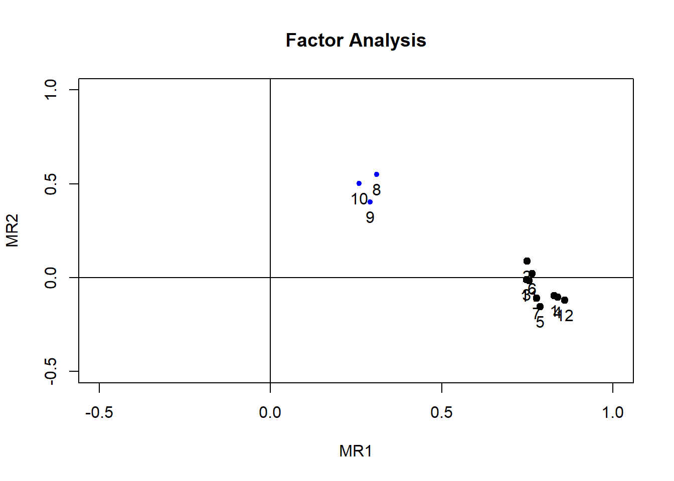
The loadings plot visualizes the un-rotated solution. While items 1-7 and 11-12 cluster together and load exclusively on Factor 1, items 8, 9, and 10 (describing experiences with facilities, appointment times and location) cluster together and separately from the rest of items. They load weakly on Factor 1 and moderately on Factor 2. Considering the item content, we may interpret Factor 1 as Overall Satisfaction, and Factor 2 as Specific Satisfaction with Environment. I said “specific” because Factor 2 captures residualized variance in this un-rotated solution - the variance left over after Factor 1 was accounted for.
QUESTION 6. What is the proportion of variance explained in all items by each of the factors, and together (total variance explained)? To answer this question, look for “Proportion Var” and “Cumulative Var” entry in the output (in a small table beginning with “SS loadings”).
Step 7. Interpreting the 2-factor orthogonally rotated solution
The objective of factor rotations is usually to simplify the un-rotated solution, so that a solution is found in which all variables are factorially simple (load on only one factor) because such models are easier to interpret. Because of simpler mathematics, orthogonal rotations were once very popular. They keep the factor axes orthogonal to each other, so that the factors remain uncorrelated.
We will now attempt to rotate the 2-factor solution orthogonally, using the popular “varimax” rotation.
##
## Loadings:
##         MR1   MR2
## esqp_01 0.820 0.159
## esqp_02 0.687 0.311
## esqp_03 0.716 0.215
## esqp_04 0.832 0.155
## esqp_05 0.797
## esqp_06 0.722 0.252
## esqp_07 0.774 0.130
## esqp_08 0.129 0.619
## esqp_09 0.155 0.473
## esqp_10       0.556
## esqp_11 0.725 0.214
## esqp_12 0.856 0.145
##
##                  MR1   MR2
## SS loadings    5.413 1.264
## Proportion Var 0.451 0.105
## Cumulative Var 0.451 0.556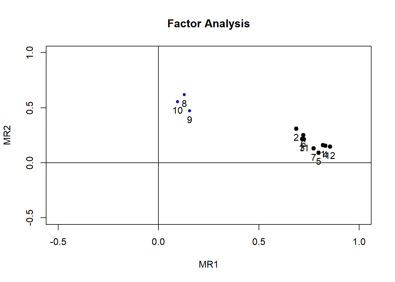
As we can see, the “varimax” rotation led to smaller loadings of items 8, 9 and 10 on Factor 1 than in the un-rotated solution. However, other cross-loadings have increased in this solution, and the items are not factorially simple as we hoped. In fact, this solution is more difficult to interpret than the un-rotated solution.
QUESTION 7. What is the proportion of variance explained in all items by each of the factors, and together (total variance explained)? To answer this question, look for “Proportion Var” and “Cumulative Var” entry in the output (in a small table beginning with “SS loadings”). Why is the total (cumulative) variance the same as in the un-rotated solution?
Step 8. Interpreting the 2-factor obliquely rotated solution
We will now try an obliquely rotated solution, using the default “oblimin” rotation.
##
## Loadings:
##         MR1    MR2
## esqp_01  0.842
## esqp_02  0.670  0.172
## esqp_03  0.721
## esqp_04  0.856
## esqp_05  0.832
## esqp_06  0.719  0.102
## esqp_07  0.799
## esqp_08         0.627
## esqp_09         0.466
## esqp_10         0.568
## esqp_11  0.731
## esqp_12  0.883
##
##                  MR1   MR2
## SS loadings    5.578 0.992
## Proportion Var 0.465 0.083
## Cumulative Var 0.465 0.547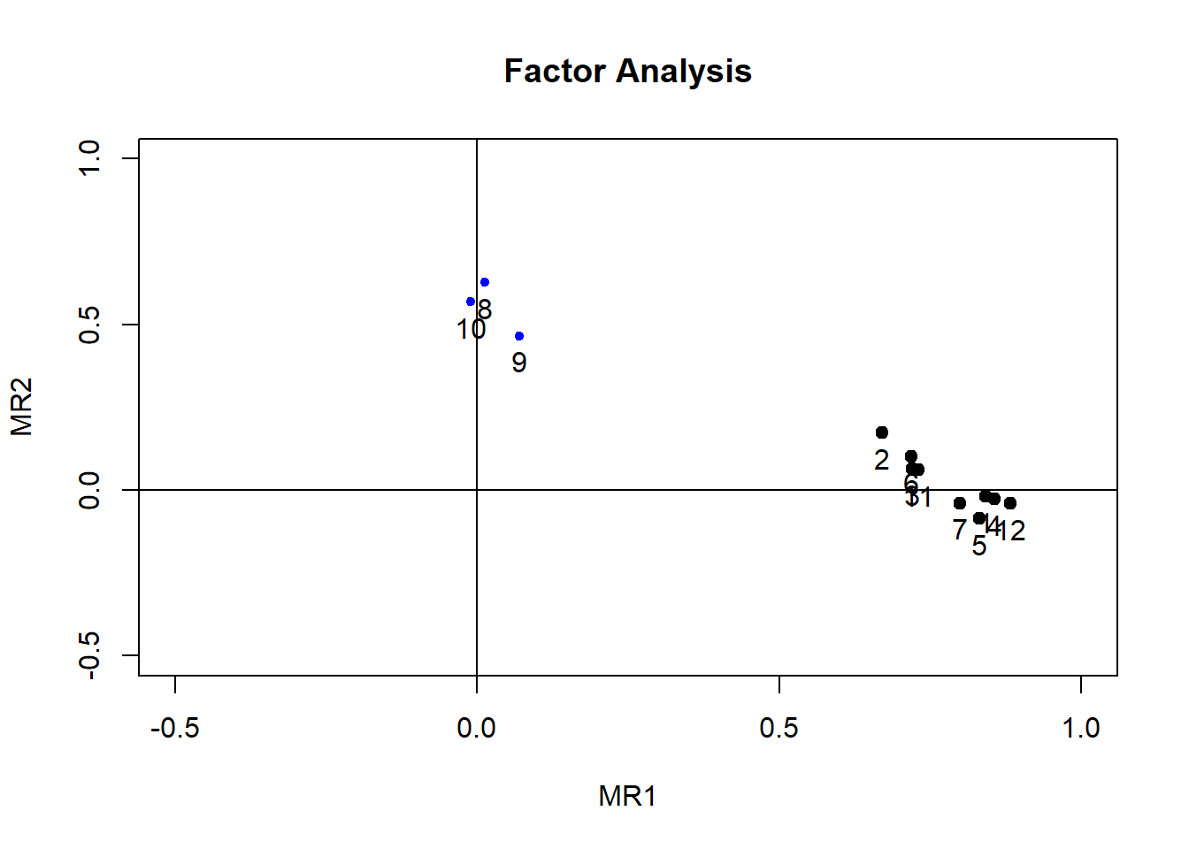
This obliquely rotated solution yields more factorially simple items than the previous solutions and is easy to interpret. Factor 1 is comprised from items 1-7 and 11-12, with the marker item esqp_12 (overall good service). Factor 2 is comprised from items 8-10, with the marker item esqp_08 (good facilities). We label the factors in this study Satisfaction with Care and Satisfaction with Environment, and these are two correlated domains of satisfaction.
QUESTION 8. What is the proportion of variance explained by each of the factors, and together (total variance explained)? To answer this question, look for “Proportion Var” and “Cumulative Var” entry in the output (in a small table beginning with “SS loadings”). Why is the total (cumulative) variance different to the one reported for the un-rotated solution?
We now ask for “Phi” - the correlation matrix of latent factors. These correlations are model-based; that is, they are estimated within the model, as one of the parameters. These correlations are between the latent factors, not their imperfect measurements (e.g. sum scores), and therefore they are the closest you can get to estimating how the actual attributes are correlated in the population. In contrast, correlations between observed sum scores will tend to be lower, because the sum scores are not perfectly reliable and correlation between them will be attenuated by unreliabilty.
##           MR1       MR2
## MR1 1.0000000 0.3876848
## MR2 0.3876848 1.0000000
QUESTION 9. Try to interpret the factor correlation matrix.
Step 9. Saving your work
After you finished work with this exercise, save your R script by pressing the Save icon in the script window. To keep all the created objects (such as fit2.o), which might be useful when revisiting this exercise, save your entire work space. To do that, when closing the project by pressing File / Close project, make sure you select Save when prompted to save your “Workspace image”.
9.4 Solutions
Q1. MSA = 0.92. According to Kaiser’s guidelines, the data are “marvellous” for fitting a factor model. Refer to Exercise 7 to remind yourself of this index and its interpretation.
Q2. There is a very sharp drop from factor #1 to factor #2, and a less pronounced drop from #2 to #3. Presumably, we have one very strong factor (presumably general satisfaction with service), which explains the general positive manifold in the correlation matrix, and 1 further factor, making 2 factors altogether. Parallel analysis confirms that 2 factors of the blue plot (observed data) are above the red dotted line (the simulated random data).
Q3. Chi-square = 394 (df=43) with prob < 3e-58. The p value is given in the scientific format, with 3 multiplied by 10 to the power of -58. It is so small (divided by 10 to the power of 58) that we can just say p<0.001. We should reject the model, because the probability of observing the given correlation matrix in the population where the 1-factor model is true (the hypothesis we are testing) is vanishingly small (p<0.001). However, chi-square test is very sensitive to the sample size, and our sample is quite large. We must judge the fit based on other criteria, for instance residuals.
Q4. The RMSR=0.04 is nice and small, indicating that the 2-factor model reproduces the observed correlations well overall.
Q5. Most residuals are very small (close to zero), and only 2 residuals are above 0.1 in absolute value. The largest residual 0.12 is between items esqp_02 and esqp_03. This is still only very slightly above 0.1. We conclude that none of the residuals cause particular concern.
Q6. In the un-rotated solution, Factor 1 accounts for 49% of total variance and Factor 2 accounts for 6.6%. As the factors are uncorrelated, these can be added together to obtain 55.6%.
Q7. After the varimax rotation, Factor 1 accounts for 45.1% of total variance and Factor 2 accounts for 10.5%. As the factors are still uncorrelated, these can be added together to obtain 55.6%. This is the same amount as in the un-rotated solution because factor rotations do not alter the total variance explained by factors in items (item uniqueness are invariant to rotation). Despite the amounts of variance re-distributing between factors, the total is still the same.
Q8. After the oblimin rotation, Factor 1 accounts for 46.5% of total variance and Factor 2 accounts for 8.3%. The cumulative total given, 54.7%, is no longer the same as in the un-rotated solution because the factors are correlated, and their variances cannot be added. However, the true total variance explained is still 55.6%, as reported in the un-rotated solution, because factor rotation does not change this result.
Q9. In the oblique solution, factors correlate moderately at 0.39. We would expect domains of satisfaction to correlate. We interpret this result as the expected correlation between constructs Satisfaction with Care and Satisfaction with Environment in the population of parents from which we sampled.