Exercise 6 Item analysis and reliability analysis of dichotomous questionnaire data
| Data file | EPQ_N_demo.txt |
| R package | psych |
6.1 Objectives
The objective of this exercise is to conduct reliability analyses on a questionnaire compiled from dichotomous items, and learn how to compute the Standard Error of measurement and confidence intervals around the observed score.
6.2 Personality study using Eysenck Personality Questionnaire (EPQ)
The Eysenck Personality Questionnaire (EPQ) is a personality inventory designed to measure Extraversion (E), Neuroticism/Anxiety (N), Psychoticism (P), and including a Social Desirability scale (L) (Eysenck and Eysenck, 1976).
The EPQ includes 90 items, to which respondents answer either “YES” or “NO” (thus giving dichotomous or binary responses). This is relatively unusual for personality questionnaires, which typically employ Likert scales to boost the amount of information from each individual item, and therefore get away with fewer items overall. On the contrary, the EPQ scales are measured by many items, ensuring a good content coverage of all domains involved. The use of binary items avoids problems with response biases such as “central tendency” (tendency to choose middle response options) and “extreme responding” (tendency to choose extreme response options).
The data were collected in the USA back in 1997 as part of a large cross-cultural study (Barrett, Petrides, Eysenck & Eysenck, 1998). This was a large study, N = 1,381 (63.2% women and 36.8% men). Most participants were young people, median age 20.5; however, there were adults of all ages present (range 16 – 89 years).
6.3 Worked Example - Reliability analysis of EPQ Neuroticism/Anxiety (N) scale
The focus of our analysis here will be the Neuroticism/Anxiety (N) scale, measured by 23 items:
N_3 Does your mood often go up and down?
N_7 Do you ever feel "just miserable" for no reason?
N_12 Do you often worry about things you should not have done or said?
N_15 Are you an irritable person?
N_19 Are your feelings easily hurt?
N_23 Do you often feel "fed-up"?
N_27 Are you often troubled about feelings of guilt?
N_31 Would you call yourself a nervous person?
N_34 Are you a worrier?
N_38 Do you worry about awful things that might happen?
N_41 Would you call yourself tense or "highly-strung"?
N_47 Do you worry about your health?
N_54 Do you suffer from sleeplessness?
N_58 Have you often felt listless and tired for no reason?
N_62 Do you often feel life is very dull?
N_66 Do you worry a lot about your looks?
N_68 Have you ever wished that you were dead?
N_72 Do you worry too long after an embarrassing experience?
N_75 Do you suffer from "nerves"?
N_77 Do you often feel lonely?
N_80 Are you easily hurt when people find fault with you or the work you do?
N_84 Are you sometimes bubbling over with energy and sometimes very sluggish?
N_88 Are you touchy about some things?
Please note that all items indicate “Neuroticism” rather than “Emotional Stability” (i.e. there are no counter-indicative items).
Step 1. Preliminary examination of the data
Because you will work with these data again, I recommend you create a new project, which you will be able to revisit later. Create a new folder with a name that you can recognize later (e.g. “EPQ Neuroticism”), and download the data file EPQ_N_demo.txt into this folder. In RStudio, create a new project in the folder you have just created. Create a new script, where you will be typing all your commands, and which you will save at the end.
The data for this exercise is not in the “native” R format, but in a tab-delimited text file with headings (you can open it in Notepad to see how it looks). You will use function read.delim() to import it into R. The function has the following general format: read.delim(file, header = TRUE, sep = "\t", ...). You must supply the first argument - the file name. Other arguments all have defaults, so you specify them only if necessary. Our file has headers and is separated by tabulation ("\t") so the defaults are just fine.
Let’s import the data into into a new object (data frame) called EPQ:
The object EPQ should appear on the Environment tab. Click on it and the data will be displayed on a separate tab. As you can see, there are 26 variables in this data frame, beginning with participant id, age and sex (0 = female; 1 = male). These demographic variables are followed by 23 item responses, which are either 0 (for “NO”) or 1 (for “YES”). There are also a few missing responses, marked with NA.
Step 2. Computing item statistics
Analyses in this Exercise will require package psych, so type and run this command from your script:
Let’s start the analyses. First, let’s call function describe() of package psych, which will print descriptive statistics for item responses in the EPQ data frame useful for psychometrics. Note that the 23 item responses start in the 4th column of the data frame.
##      vars    n mean   sd median trimmed mad min max range  skew kurtosis   se
## N_3     1 1379 0.64 0.48      1    0.67   0   0   1     1 -0.57    -1.67 0.01
## N_7     2 1379 0.54 0.50      1    0.56   0   0   1     1 -0.18    -1.97 0.01
## N_12    3 1381 0.80 0.40      1    0.87   0   0   1     1 -1.47     0.17 0.01
## N_15    4 1375 0.29 0.45      0    0.24   0   0   1     1  0.93    -1.13 0.01
## N_19    5 1377 0.58 0.49      1    0.60   0   0   1     1 -0.31    -1.90 0.01
## N_23    6 1377 0.51 0.50      1    0.52   0   0   1     1 -0.06    -2.00 0.01
## N_27    7 1377 0.47 0.50      0    0.47   0   0   1     1  0.11    -1.99 0.01
## N_31    8 1378 0.33 0.47      0    0.29   0   0   1     1  0.70    -1.51 0.01
## N_34    9 1378 0.60 0.49      1    0.62   0   0   1     1 -0.41    -1.84 0.01
## N_38   10 1378 0.53 0.50      1    0.54   0   0   1     1 -0.13    -1.99 0.01
## N_41   11 1370 0.31 0.46      0    0.26   0   0   1     1  0.83    -1.30 0.01
## N_47   12 1380 0.58 0.49      1    0.60   0   0   1     1 -0.33    -1.89 0.01
## N_54   13 1378 0.31 0.46      0    0.27   0   0   1     1  0.80    -1.36 0.01
## N_58   14 1381 0.66 0.47      1    0.70   0   0   1     1 -0.67    -1.56 0.01
## N_62   15 1380 0.27 0.45      0    0.22   0   0   1     1  1.02    -0.97 0.01
## N_66   16 1378 0.58 0.49      1    0.60   0   0   1     1 -0.34    -1.89 0.01
## N_68   17 1379 0.44 0.50      0    0.42   0   0   1     1  0.26    -1.93 0.01
## N_72   18 1379 0.61 0.49      1    0.64   0   0   1     1 -0.45    -1.80 0.01
## N_75   19 1375 0.36 0.48      0    0.32   0   0   1     1  0.59    -1.66 0.01
## N_77   20 1376 0.41 0.49      0    0.39   0   0   1     1  0.35    -1.88 0.01
## N_80   21 1375 0.61 0.49      1    0.64   0   0   1     1 -0.45    -1.80 0.01
## N_84   22 1376 0.81 0.39      1    0.89   0   0   1     1 -1.58     0.48 0.01
## N_88   23 1376 0.89 0.31      1    0.99   0   0   1     1 -2.51     4.29 0.01
QUESTION 1. Examine the output. Look for the descriptive statistic representing item difficulty. Do the difficulties vary widely? What is the easiest (to agree with) item in this set? What is the most difficult (to agree with) item? Examine phrasing of the corresponding items – can you see why one item is easier to agree with than the other?
Now let’s compute the product-moment (Pearson) correlations between EPQ items using function lowerCor() of package psych. This function is very convenient because, unlike the base R function cor(), it shows only the lower triangle of the correlation matrix, which is more compact and easier to read. If you call help on this function you will see that by default the correlations will be printed to 2 decimal places (digits=2), and the missing values will be treated in the pairwise fashion (use="pairwise"). This is good, and we will not change any defaults.
Now let’s compute the tetrachoric correlations for the same items. These would be more appropriate for binary items on which a NO/YES dichotomy was forced (although the underlying extent of agreement is actually continuous). The function tetrachoric() has the pairwise deletion for missing values by default - again, this is good.
QUESTION 2. Examine the outputs for product-moment and tetrachoric correlations. Compare them to each other. What do you notice? How do you interpret the findings?
Step 3 (Optional). Computing the total scale score and statistics
We can compute the Neuroticism scale score (as a sum of its item scores). Note that there are no counter-indicative items in the Neuroticism scale, so there is no need to reverse code any.
From Exercise 1 you should already know that in the presence of missing data, adding the items scores is not advisable because any response will essentially be treated as zero, which is not right because not providing an answer to a question is not the same as saying “NO”.
Instead, we will again use the base R function rowMeans() to compute the average score from non-missing item responses (removing “NA” values from calculation, na.rm=TRUE), and then multiply the result by 23 (the number of items in the Neuroticism scale). This will essentially replace any missing responses with the mean for that individual, thus producing a fair estimate of the total score.
Check out the new object N_score in the Environment tab. You will see that scores for those with missing data (for example, participant #1, who had response to N_88 missing) may have decimal points and scores for those without missing data (for example, participant #2) are integers.
Now we can compute descriptive statistics for the Neuroticism score.
##    vars    n  mean   sd median trimmed  mad min max range  skew kurtosis   se
## X1    1 1381 12.15 5.53     12   12.17 5.93   0  23    23 -0.03    -0.89 0.15
And we plot the histogram, which will appear in the “Plots” tab:
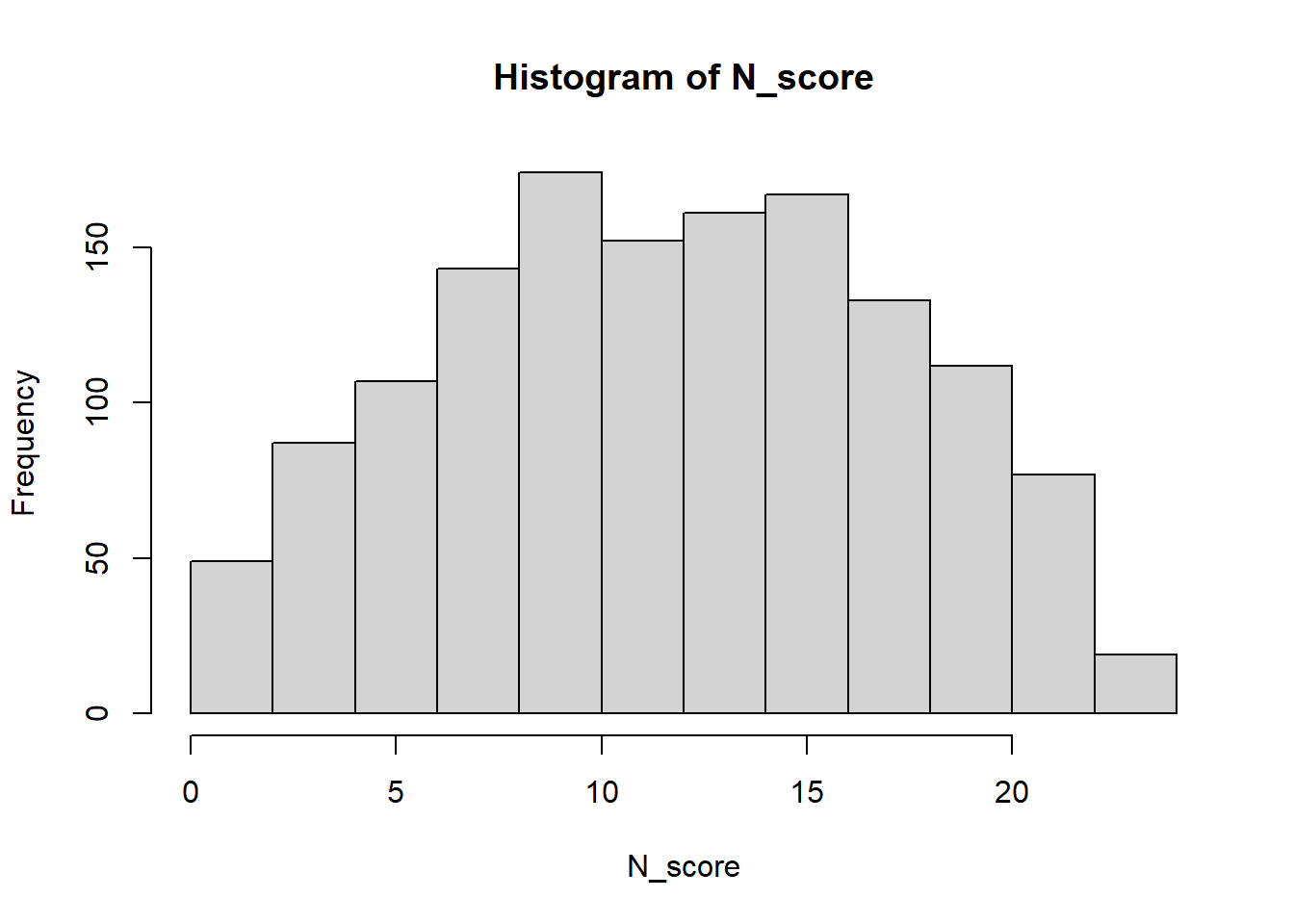
QUESTION 3. Examine the histogram. What can you say about the test difficulty for the tested population?
Step 4. Estimating the coefficient alpha based on product-moment correlations
Now let’s estimate the “internal consistency reliability” (Cronbach’s alpha) of the total score. We apply function alpha() from the psych package to all 23 items of the SDQ data frame. Like in Exercise 5, I suggest obtaining output for the sum score (which we computed) rather than average score (default in alpha()).
##
## Reliability analysis
## Call: alpha(x = EPQ[4:26], cumulative = TRUE)
##
##   raw_alpha std.alpha G6(smc) average_r S/N    ase mean  sd median_r
##       0.87      0.87    0.88      0.22 6.7 0.0049   12 5.5     0.22
##
##     95% confidence boundaries
##          lower alpha upper
## Feldt     0.86  0.87  0.88
## Duhachek  0.86  0.87  0.88
##
##  Reliability if an item is dropped:
##      raw_alpha std.alpha G6(smc) average_r S/N alpha se  var.r med.r
## N_3       0.86      0.86    0.87      0.22 6.2   0.0052 0.0075  0.21
## N_7       0.86      0.86    0.87      0.22 6.3   0.0052 0.0075  0.21
## N_12      0.87      0.86    0.87      0.22 6.4   0.0051 0.0075  0.22
## N_15      0.87      0.87    0.87      0.23 6.5   0.0050 0.0074  0.22
## N_19      0.86      0.86    0.87      0.22 6.2   0.0053 0.0067  0.21
## N_23      0.86      0.86    0.87      0.22 6.2   0.0052 0.0075  0.21
## N_27      0.86      0.86    0.87      0.22 6.3   0.0052 0.0075  0.21
## N_31      0.86      0.86    0.87      0.22 6.3   0.0052 0.0068  0.22
## N_34      0.86      0.86    0.87      0.22 6.1   0.0053 0.0067  0.21
## N_38      0.86      0.86    0.87      0.22 6.3   0.0052 0.0075  0.21
## N_41      0.87      0.86    0.87      0.22 6.3   0.0051 0.0072  0.22
## N_47      0.87      0.87    0.88      0.23 6.6   0.0049 0.0071  0.23
## N_54      0.87      0.87    0.88      0.23 6.6   0.0050 0.0073  0.23
## N_58      0.87      0.86    0.87      0.22 6.4   0.0051 0.0076  0.22
## N_62      0.87      0.87    0.87      0.23 6.4   0.0051 0.0074  0.22
## N_66      0.87      0.87    0.87      0.23 6.5   0.0050 0.0075  0.22
## N_68      0.87      0.87    0.87      0.23 6.5   0.0050 0.0075  0.23
## N_72      0.86      0.86    0.87      0.22 6.3   0.0052 0.0070  0.21
## N_75      0.86      0.86    0.87      0.22 6.2   0.0052 0.0070  0.21
## N_77      0.86      0.86    0.87      0.22 6.2   0.0052 0.0074  0.21
## N_80      0.87      0.86    0.87      0.22 6.3   0.0052 0.0069  0.22
## N_84      0.87      0.87    0.88      0.23 6.6   0.0050 0.0071  0.23
## N_88      0.87      0.87    0.88      0.23 6.7   0.0050 0.0068  0.23
##
##  Item statistics
##         n raw.r std.r r.cor r.drop mean   sd
## N_3  1379  0.58  0.58  0.56   0.52 0.64 0.48
## N_7  1379  0.56  0.56  0.54   0.50 0.54 0.50
## N_12 1381  0.49  0.50  0.46   0.43 0.80 0.40
## N_15 1375  0.44  0.44  0.40   0.37 0.29 0.45
## N_19 1377  0.61  0.61  0.60   0.56 0.58 0.49
## N_23 1377  0.58  0.58  0.55   0.51 0.51 0.50
## N_27 1377  0.57  0.57  0.54   0.51 0.47 0.50
## N_31 1378  0.55  0.55  0.53   0.49 0.33 0.47
## N_34 1378  0.64  0.64  0.63   0.59 0.60 0.49
## N_38 1378  0.56  0.55  0.52   0.49 0.53 0.50
## N_41 1370  0.52  0.52  0.49   0.46 0.31 0.46
## N_47 1380  0.37  0.37  0.32   0.29 0.58 0.49
## N_54 1378  0.39  0.39  0.34   0.31 0.31 0.46
## N_58 1381  0.51  0.51  0.48   0.44 0.66 0.47
## N_62 1380  0.46  0.46  0.43   0.40 0.27 0.45
## N_66 1378  0.45  0.44  0.40   0.37 0.58 0.49
## N_68 1379  0.44  0.44  0.39   0.37 0.44 0.50
## N_72 1379  0.57  0.57  0.54   0.51 0.61 0.49
## N_75 1375  0.59  0.58  0.57   0.52 0.36 0.48
## N_77 1376  0.58  0.58  0.55   0.52 0.41 0.49
## N_80 1375  0.54  0.54  0.52   0.47 0.61 0.49
## N_84 1376  0.35  0.37  0.31   0.29 0.81 0.39
## N_88 1376  0.30  0.33  0.27   0.25 0.89 0.31
##
## Non missing response frequency for each item
##         0    1 miss
## N_3  0.36 0.64 0.00
## N_7  0.46 0.54 0.00
## N_12 0.20 0.80 0.00
## N_15 0.71 0.29 0.00
## N_19 0.42 0.58 0.00
## N_23 0.49 0.51 0.00
## N_27 0.53 0.47 0.00
## N_31 0.67 0.33 0.00
## N_34 0.40 0.60 0.00
## N_38 0.47 0.53 0.00
## N_41 0.69 0.31 0.01
## N_47 0.42 0.58 0.00
## N_54 0.69 0.31 0.00
## N_58 0.34 0.66 0.00
## N_62 0.73 0.27 0.00
## N_66 0.42 0.58 0.00
## N_68 0.56 0.44 0.00
## N_72 0.39 0.61 0.00
## N_75 0.64 0.36 0.00
## N_77 0.59 0.41 0.00
## N_80 0.39 0.61 0.00
## N_84 0.19 0.81 0.00
## N_88 0.11 0.89 0.00
QUESTION 4. What is alpha for the Neuroticism scale score? Report the raw_alpha printed at the beginning of the output (this is the version of alpha calculated from row item scores and covariances rather than standardized item scores and correlations).
Examine the alpha() output further. You can call ?alpha to get help on this function and its output. An important summary statistic is average_r, which stands for the average inter-item correlation. Other useful summary statistics are mean and sd, which are respectively the mean and the standard deviation of the test score. Yes, you can get these statistics without computing the test score by just running function alpha(). Isn’t this convenient?
If you completed Step 3, and computed N_score previously and obtained its mean and SD using function describe(N_score), you can now compare these results. The mean and SD given in alpha() should be the same (maybe rounded to fewer decimal points) as the results from describe().
In the “Item statistics” output, an interesting statistic is r.drop – that is the correlation between the item score and the total score with this particular item dropped. This tells you how closely each item is associated with the remaining items. The higher this value is, the more representative the item is of the whole item collection.
QUESTION 5. Which item has the highest correlation with the remaining items (r.drop value)? Look up this item’s content in the EPQ questionnaire.
In “Reliability if an item is dropped” output, an important statistic is raw_alpha. It tells you how the scale’s alpha would change if you dropped a particular item. If an item contributes information to measurement, its “alpha if deleted” should be lower than the actual alpha (this might not be obvious as the values might be different in the third decimal point). In this questionnaire, dropping any item will not reduce the alpha by more than 0.01. This is not surprising since the scale is long (consists of 23 items), and dropping one item is not going to reduce the reliability dramatically.
Step 5. Estimating the coefficient alpha based on tetrachoric correlations
Now, remember that in the standard alpha computation, the product-moment covariances are used (the basis for Pearson’s correlation coefficient). These assume continuous data and typically underestimate the degree of relationship between binary “YES/NO” items, so a better option would be to compute alpha from tetrachoric correlations. We have already used function tetrachoric() to compute the tetrachoric correlations for the EPQ items. Please examine the output of that function again carefully. You should see that this function returns the matrix of correlations (which we will need) as well as thresholds or “tau” (which we won’t). Let’s run the function again, this time assigning its results to a new object EPQtetr:
Press on the little blue arrow next to EPQtetr in the Environment tab. The object’s structure will be revealed and you should see that EPRtetr contains rho, which is is a 23x23 matrix of the tetrachoric correlations, tau, which is the vector of 23 thresholds, etc. To retrieve the tetrachoric correlations from the object EPQtetr, we can simply refer to them like so EPQtetr$rho.
Now you can pass the tetrachoric correlations to function alpha(). Note that because you pass the correlations rather than the raw scores, no statistics for the “test score” can be computed and you cannot specify the type of score using the cumulative option.
##
## Reliability analysis
## Call: alpha(x = EPQtetr$rho)
##
##   raw_alpha std.alpha G6(smc) average_r S/N median_r
##       0.93      0.93    0.95      0.37  13     0.36
##
##     95% confidence boundaries
##       lower alpha upper
## Feldt  0.88  0.93  0.97
##
##  Reliability if an item is dropped:
##      raw_alpha std.alpha G6(smc) average_r S/N var.r med.r
## N_3       0.93      0.93    0.94      0.36  12 0.015  0.35
## N_7       0.93      0.93    0.94      0.36  13 0.015  0.35
## N_12      0.93      0.93    0.94      0.37  13 0.014  0.36
## N_15      0.93      0.93    0.94      0.37  13 0.014  0.37
## N_19      0.93      0.93    0.94      0.36  12 0.013  0.35
## N_23      0.93      0.93    0.94      0.36  13 0.015  0.35
## N_27      0.93      0.93    0.94      0.36  13 0.015  0.35
## N_31      0.93      0.93    0.94      0.37  13 0.013  0.36
## N_34      0.92      0.92    0.94      0.36  12 0.013  0.35
## N_38      0.93      0.93    0.94      0.37  13 0.015  0.35
## N_41      0.93      0.93    0.94      0.37  13 0.014  0.36
## N_47      0.93      0.93    0.95      0.38  13 0.013  0.38
## N_54      0.93      0.93    0.95      0.38  13 0.014  0.38
## N_58      0.93      0.93    0.94      0.37  13 0.015  0.37
## N_62      0.93      0.93    0.94      0.37  13 0.014  0.37
## N_66      0.93      0.93    0.95      0.37  13 0.015  0.37
## N_68      0.93      0.93    0.95      0.37  13 0.014  0.37
## N_72      0.93      0.93    0.94      0.36  13 0.014  0.35
## N_75      0.93      0.93    0.94      0.36  13 0.014  0.35
## N_77      0.93      0.93    0.94      0.36  13 0.014  0.35
## N_80      0.93      0.93    0.94      0.37  13 0.014  0.36
## N_84      0.93      0.93    0.95      0.38  13 0.014  0.37
## N_88      0.93      0.93    0.95      0.38  13 0.014  0.38
##
##  Item statistics
##         r r.cor r.drop
## N_3  0.72  0.71   0.69
## N_7  0.68  0.67   0.64
## N_12 0.66  0.65   0.62
## N_15 0.56  0.54   0.51
## N_19 0.74  0.74   0.70
## N_23 0.70  0.69   0.66
## N_27 0.69  0.67   0.65
## N_31 0.67  0.67   0.63
## N_34 0.78  0.78   0.75
## N_38 0.67  0.65   0.63
## N_41 0.65  0.64   0.61
## N_47 0.44  0.40   0.38
## N_54 0.48  0.44   0.42
## N_58 0.63  0.62   0.59
## N_62 0.59  0.57   0.54
## N_66 0.54  0.50   0.48
## N_68 0.53  0.50   0.48
## N_72 0.68  0.67   0.65
## N_75 0.72  0.71   0.68
## N_77 0.70  0.69   0.66
## N_80 0.65  0.64   0.60
## N_84 0.49  0.46   0.43
## N_88 0.48  0.45   0.43
QUESTION 6. What is the tetrachoric-based alpha and how does it compare to alpha computed from product-moment covariances?
Step 6. Computing the Standard Error of measurement for the total score
Finally, let’s compute the Standard Error of measurement from the tetrachorics-based alpha using the formula
SEm(y) = SD(y)*sqrt(1-alpha)You will need the standard deviation of the total score, which you already computed (scroll up your output to the descriptives for N_score). Now you can substitute the SD value and also the alpha value into the formula, and do the calculation in R by typing them in your script and then running them in the Console.
## [1] 1.4631Even better would be to save the result in a new object SEm, so we can use it later for computing confidence intervals.
QUESTION 7. As a challenge, try to compute the SEm not by substituting the value for standard deviation from the previous output, but by computing the standard deviation of N_score from scratch using base R function sd().
Step 7. Computing the Confidence Interval around a score
Finally, let’s compute the 95% confidence interval around a given score Y using formulas Y-2*SEm and Y+2*SEm. Say, we want to compute the 95% confidence interval around N_score for Participant #1. It is easy to pull out the respective score from vector N_score (which holds scores for 1381 participants) by simply referring to the participant number in square brackets: N_score[1].
QUESTION 8. What is the 95% confidence interval around the Neuroticism scale score for participant #1?
6.4 Solutions
Q1. The mean represents item difficulty. In this item set, difficulties vary widely. The ‘easiest’ item to endorse is N_88 (“Are you touchy about some things?”), with the highest mean (0.89). Because the data are binary coded 0/1, the mean can be interpreted as 89% of the sample endorsed the item. The most difficult item to endorse in this set is N_62, with the lowest mean value (0.27). N_62 is phrased “Do you often feel life is very dull?”, and only 27% of the sample agreed with this. This item indicates a higher degree of Neuroticism (perhaps even a symptom of depression) than that of item N_88, and it is therefore more difficult to endorse.
Q2. The tetrachoric correlations are substantially larger than the product-moment correlations. This is not surprising given that the data are binary and the product-moment correlations were developed for continuous data. The product-moment correlations underestimate the strength of the relationships between these binary items.
Q3. The distribution appears symmetrical, without any visible skew. There is no ceiling or floor effects, so the test’s difficulty appears appropriate for the population.
Q4. The (raw) alpha computed from product-moment covariances is 0.87.
Q5. Item N_34 (“Are you a worrier?”) has the highest item-total correlation (when the item itself is dropped). This item is central to the meaning of the scale, or, in other words, the item that best represents this set of items. This makes sense given that the scale is supposed to measure Neuroticism. Worrying about things is one of core indicators of Neuroticism.
Q6. Alpha from tetrachoric correlations is 0.93. It is larger than the product-moment based alpha. This is not surprising since the tetrachoric correlations were greater than the product-moment correlations.
Q7.
## [1] 1.463404Q8. The 95% confidence interval is (9.62, 15.47)
## [1] 9.618647## [1] 15.47226