Exercise 1 Likert scaling of ordinal questionnaire data, creating a sum score, and norm referencing
| Data file | SDQ.RData |
| R package | psych |
1.1 Objectives
The purpose of this exercise is to learn how to compute test scores from ordinal test responses, and interpret them in relation to a norm. You will also learn how to deal with missing responses when computing test scores.
You will also learn how to deal with items that indicate the opposite end of the construct to other items. Such items are sometimes called “negatively keyed” or “counter-indicative”. Compare, for example, item “I get very angry and often lose my temper” with item “I usually do as I am told”. They represent positive and negative indicators of Conduct Problems, respectively. The (small) problem with such items is that they need to be appropriately coded before computing the test score so that the score unambiguously reflects “problems” rather than the lack thereof. This exercise will show you how to do that.
1.2 Study of a community sample using the Strength and Difficulties Questionnaire (SDQ)
The Strengths and Difficulties Questionnaire (SDQ) is a brief behavioural screening questionnaire about children and adolescents of 3-16 years of age. It exists in several versions to meet the needs of researchers, clinicians and educationalists, see http://www.sdqinfo.org/. You can download the questionnaire, and also the scoring key and norms provided by the test publisher.
The self-rated (SDQ Pupil) version includes 25 items measuring 5 scales (facets), with 5 items each:
| Emotional Symptoms | somatic | worries | unhappy | clingy | afraid |
| Conduct Problems | tantrum | obeys* | fights | lies | steals |
| Hyperactivity | restles | fidgety | distrac | reflect* | attends* |
| Peer Problems | loner | friend* | popular* | bullied | oldbest |
| Pro-social | consid | shares | caring | kind | helpout |
Respondents are asked to rate each question using the following response options: 0 = “Not true” 1 = “Somewhat true” 2 = “Certainly true”
NOTE that some SDQ items represent behaviours counter-indicative of the scales they intend to measure, so that higher scale scores correspond to lower item scores. For instance, item “I usually do as I am told” (variable obeys) is counter-indicative of Conduct Problems. There are 5 such items in the SDQ; they are marked in the above table with asterisks (*).
Participants in this study are year 7 pupils from the same school (N=228). This is a community sample, and we do not expect many children to have scores above clinical thresholds. The SDQ was administered twice, the first time when the children just started secondary school (were in Year 7), and one year later (were in year 8).
1.3 Worked Example 1 - Likert scaling and norm referencing for Emotional Symptoms scale
This worked example is analysis of the first SDQ scale, Emotional Symptoms. This scale has no counter-indicative items.
Step 1. Preliminary examination of data set
If you downloaded the file SDQ.RData and saved it in the same folder as this project, you should see the file name in the Files tab (usually in the bottom right RStudio panel). Now we can load an object (data frame) contained in this “native” R file (with extension .RData) into RStudio using the basic function load().
You should see a new object SDQ appear on the Environment tab (top right RStudio panel). This tab will show any objects currently in the workspace, and the data frame SDQ was stored in file SDQ.RData we just loaded. According to the description in the Environment tab, the data frame contains “228 obs.” (observations) “of 51 variables”; that is, 228 rows and 51 columns.
You can press on the SDQ object. You should see the View(SDQ) command run on Console, and, in response to that command, the data set should open up in its own tab named SDQ. Examine the data by scrolling down and across. The data set contains 228 rows (cases, observations) on 51 variables. There is a Gender variable (0=male; 1=female), followed by responses to 25 SDQ items named consid, restles, somatic etc. (these are variable names in the order of items in the questionnaire). Item variables reflect the key meaning of the actual SDQ questions, which are also attached to the data frame as labels. For example, consid is a shortcut for “I try to be nice to other people. I care about their feelings”, or restles is a shortcut for “I am restless, I cannot stay still for long”. These 25 variables are followed by 25 more variables named consid2, restles2, somatic2 etc. These are responses to the same SDQ items at Time 2.
You should also see that there are some missing responses, marked ‘NA’. There are more missing responses for Time 2, with whole rows missing for some pupils. This is typical for longitudinal data, because it is not always possible to obtain responses from the same pupil one year later (for example, the pupil might have moved schools).
You can obtain the names of all variables by typing and running command names(SDQ).
Step 2. Creating variable lists
Let us start analysis by creating a list of items that measure Emotional Symptoms (you can see them in a table given earlier). This will enable easy reference to data from these 5 items (variables) in all analyses. We will use c() - the base R function for combining values into a list.
Note how a new object items_emotion appeared in the Environment tab. Now you will be able to refer only to data from these variables by referring to SDQ[items_emotion]. Try running this command and see how you get only responses to the 5 items we specified.
QUESTION 1. Now use the same logic to create a list of items measuring Emotional Symptoms at Time 2, called items_emotion2.
Step 3. Computing the test score
Now you are ready to compute the Emotional Symptoms scale score for Time 1. Normally, we could use the base R function rowSums(), which computes the sum of specified variables for each row (pupil):
##   [1]  4  3  1  2  4  2  4  0  1  1  0  8  2  3  7  4  5  2  8  6  1  4  9  4  5
##  [26]  9  0  3  3  1  0  2  6  3  9  4  4  0  7  1  3  6  4  5  4  1  4  1  0  5
##  [51]  1  2  2  4  4  4  6  1  8  3  2  2  4  1  1  0  2  2  7  5  0 NA NA  1  1
##  [76]  7  4  1  8  3  5  0  5  4  0  1  1  5  3  6  1  3  2  6  6  0  2  4  5  3
## [101]  3  1  1  7  2  3  5  5 NA  0  4  0  4  1  1  1  1  0  2  7  0  3  8  4  6
## [126] NA  2  4  7  1  0  0  1  0  4  3  0 10  5  2  1  6  1  2  1  0  1 NA  4  4
## [151]  2  4  7  5  6  1  0  5  3  1  3  3  6  4  2  3  1  0  3  3  0  3  0  0  0
## [176]  2  2  2  0  1  5  3  3  1  4  3  1  6  2  4  2 NA  0  2  5  5  0  2  2  3
## [201]  4  0  2  4  2  2  1  3  2  0  1  0  0  8  1  1  2  1  2  2  4  0  0  1  2
## [226]  2  1  6
Try this and check out the resulting scores printed in the Console window. Oops! It appears that pupils with missing responses (even on one item) got ‘NA’ for their scale score. This is because the default option for dealing with missing data in the rowSums() function is to skip any rows with missing data. Let’s change to skipping only the ‘NA’ responses, not whole rows, like so:
##   [1]  4  3  1  2  4  2  4  0  1  1  0  8  2  3  7  4  5  2  8  6  1  4  9  4  5
##  [26]  9  0  3  3  1  0  2  6  3  9  4  4  0  7  1  3  6  4  5  4  1  4  1  0  5
##  [51]  1  2  2  4  4  4  6  1  8  3  2  2  4  1  1  0  2  2  7  5  0  2  7  1  1
##  [76]  7  4  1  8  3  5  0  5  4  0  1  1  5  3  6  1  3  2  6  6  0  2  4  5  3
## [101]  3  1  1  7  2  3  5  5  4  0  4  0  4  1  1  1  1  0  2  7  0  3  8  4  6
## [126]  0  2  4  7  1  0  0  1  0  4  3  0 10  5  2  1  6  1  2  1  0  1  4  4  4
## [151]  2  4  7  5  6  1  0  5  3  1  3  3  6  4  2  3  1  0  3  3  0  3  0  0  0
## [176]  2  2  2  0  1  5  3  3  1  4  3  1  6  2  4  2  4  0  2  5  5  0  2  2  3
## [201]  4  0  2  4  2  2  1  3  2  0  1  0  0  8  1  1  2  1  2  2  4  0  0  1  2
## [226]  2  1  6
Now you should get scale scores for all pupils, but in this calculation, the missing responses are simply skipped, so essentially treated as zeros. This is not quite right. Remember that there might be different reasons for not answering a question, and not answering the question is not the same as saying “Not true”, therefore should not be scored as 0.
Instead, we will do something more intelligent. We will use the rowMeans() function to compute the mean of those item responses that are present (still skipping the ‘NA’ values, na.rm=TRUE), and then multiply the result by 5 (the number of items in the scale) to obtain a fair estimate of the sum score.
For example, if all non-missing responses of a person are 2, the mean is also 2, and multiplying this mean by the number of items in the scale, 5, will give a fair estimate of the expected scale score, 5x2=10. So we essentially replace any missing responses with the mean response for that person, thus producing a fairer test score.
Try this and compare with the previous result from rowSums(). It should give the same values for the vast majority of pupils, because they had no missing data. The only differences will be for those few pupils who had missing data.
Now we will repeat the calculation, but this time appending the resulting score as a new column (variable) named S_emotion to the data frame SDQ:
Let’s check whether the calculation worked as expected for those pupils with missing data, for example case #72. Let’s pull that specific record from the data frame, referring to the row (case) number, and then to the columns (variables) of interest:
##    somatic worries unhappy clingy afraid
## 72       0       1       0      1     NA
You can see that one response is missing on item afraid. If we just added up the non-missing responses for this pupil, we would get the scale score of 2. However, the mean of 4 non-missing scores is (0+1+0+1)/4 = 0.5, and multiplying this by the total number of items 5 should give the scale score 2.5. Now check the entry for this case in S_emotion:
## [1] 2.5QUESTION 2. Repeat the above steps to compute the test score for Emotional Symptoms at Time 2 (call it S_emotion2), and append the score to the SDQ data frame as a new column.
Step 4. Examining the distribution and scale score statistics
We start by plotting a basic histogram of the S_emotion score:
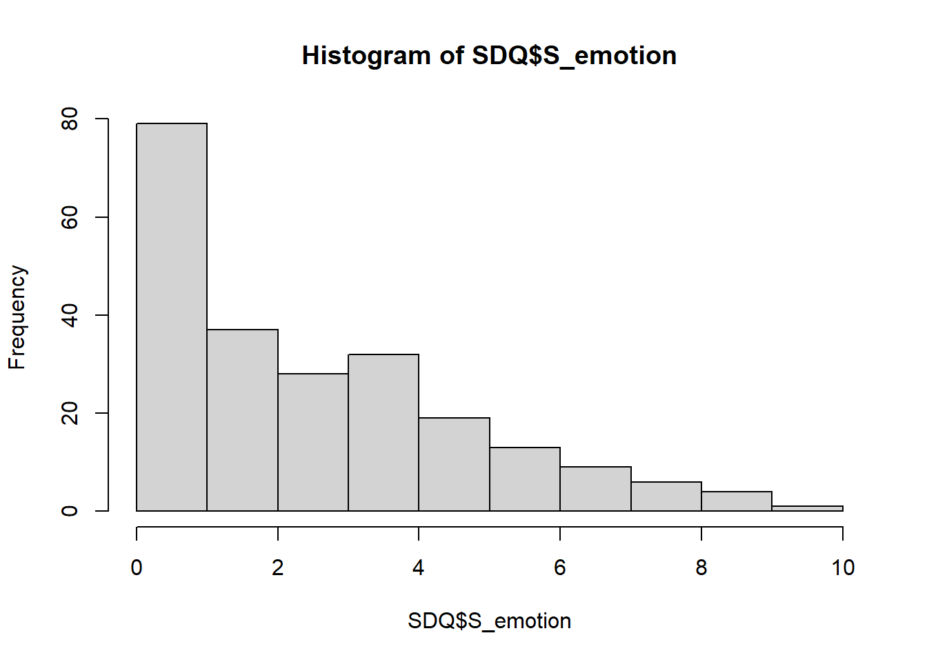
QUESTION 3. What can you say about the distribution of S_emotion score? Is the Emotional Symptoms subtest “easy” for the children in this community, or “difficult”?
You can also compute descriptive statistics for S_emotion, using a very convenient function describe()from package psych, which will give the range, the mean, the median, the standard deviation and other useful statistics.
##    vars   n mean   sd median trimmed  mad min max range skew kurtosis   se
## X1    1 228 2.89 2.33      2    2.66 2.97   0  10    10 0.72    -0.16 0.15
As you can see, the median (the score below which half of the sample lies) of S_emotion is 2, while the mean is higher at 2.89. This is because the score is positively skewed; in this case, the median is more representative of the central tendency. These statistics are consistent of our observation of the histogram, showing a profound floor effect.
QUESTION 4. Obtain and interpret the histogram and the descriptives for S_emotion2 independently.
Step 5. Norm referencing
Below are the cut-offs for “Normal”, “Borderline” and “Abnormal” cases for Emotional Symptoms provided by the test publisher (see https://sdqinfo.org/). These are the scores that set apart likely borderline and abnormal cases from the “normal” cases.
- Normal: 0-5
- Borderline: 6
- Abnormal: 7-10
Use the histogram you plotted earlier for S_emotion (Time 1) to visualize roughly how many children in this community sample fall into the “Normal”, “Borderline” and “Abnormal” bands.
Now let’s use the function table(), which tabulates cases with each score value.
##
##                0                1                2              2.5
##               36               43               37                1
##                3                4                5                6
##               27               32               19               13
## 6.66666666666667                7                8             8.75
##                1                8                6                1
##                9               10
##                3                1
A few non-integer scores must not worry you. They occurred due to computing the scale score from the item means for some pupils with missing responses. For all cases without missing responses, the resulting scale scores will be integers.
We can use the table() function to establish the number of children in this sample in the “Normal” range. From the cut-offs, we know that the Normal range is that with S_emotion score between 0 and 5. Simply specify this condition (that we want scores less or equal to 5) when calling the function:
##
## FALSE  TRUE
##    33   195
This gives 195 children or 85.5% (195/228=0.855) classified in the Normal range.
QUESTION 5. Now try to work out the percentage of children who can be classified “Borderline” on Emotional Symptoms (Time 1 only).
QUESTION 6. What is the percentage of children in the “Abnormal” range on Emotional Symptoms (Time 1 only)?
1.4 Worked Example 2 - Reverse coding counter-indicative items and computing test score for SDQ Conduct Problems
This worked example comprises scaling of the SDQ items measuring Conduct Problems. Once you feel confident with reverse coding, you can complete the exercise for the remaining SDQ facets that contain counter-indicative items.
Step 1. Creating variable list
Remind yourself about items designed to measure Conduct Problems. You can see them in a table given in Worked Example 1.3. Now let us create a list, which will enable easy reference to data from these 5 variables in all analyses.
Note how a new object items_conduct appeared in the Environment tab. Try calling SDQ[items_conduct] to pull only the data from these 5 items.
QUESTION 7. Create a list of items measuring Conduct Problems at Time 2, called items_conduct2.
Step 2. Reverse coding counter-indicative items
Before adding item scores together to obtain a scale score, we must reverse code any items that are counter-indicative to the scale. Otherwise, positive and negative indicators of the construct will cancel each other out in the sum score!
For Conduct Problems, we have only one counter-indicative item, obeys. To reverse–code this item, we will use a dedicated function of the psych package, reverse.code(). This function has the general form reverse.code(keys, items,…). Argument keys is a vector of values 1 or -1, where -1 implies to reverse the item. Argument items is the names of variables we want to score. Let’s look at the set of items again:
tantrum obeys* fights lies stealsSince the only item to reverse-code is #2 in the set of 5 items, we will combine the following values in a vector to obtain keys=c(1,-1,1,1,1). The whole command will look like this:
We assigned the appropriately coded subset of 5 items to a new object, R_conduct. Preview the item scores in this object :
##      tantrum obeys- fights lies steals
## [1,]       0      0      0    0      0
## [2,]       0      0      0    0      0
## [3,]       0      0      0    0      0
## [4,]       0      0      0    0      0
## [5,]       1      2      0    2      0
## [6,]       0      0      0    0      0
You should see that the item obeys is marked with “-“, and that it is indeed reverse coded, if you compare it with the original below. How good is that?
##   tantrum obeys fights lies steals
## 1       0     2      0    0      0
## 2       0     2      0    0      0
## 3       0     2      0    0      0
## 4       0     2      0    0      0
## 5       1     0      0    2      0
## 6       0     2      0    0      0
QUESTION 8. Use the logic above to reverse code items measuring Conduct Problems at Time 2, saving them in object R_conduct2.
Step 3. Computing the test score
Now we are ready to compute the Conduct Problems scale score for Time 1. Because there are missing responses (particularly for Time 2), we will use the rowMeans() function to compute the mean of those item responses that are present (skipping the ‘NA’ values, na.rm=TRUE), and then multiply the result by 5 (the number of items in the scale) to obtain a fair estimate of the sum score. Please refer to Worked Example 1.3 (Step 2) for a detailed explanation of this procedure.
Importantly, we will use the reverse-coded items (R_conduct) rather than original items (SDQ[items_conduct])in the calculation of the sum score. We will append the computed scale score as a new variable (column) named S_conduct to data frame SDQ:
QUESTION 9. Compute the test score for Conduct Problems at Time 2 (call it S_conduct2), and append the score to the SDQ data frame as a new variable (column).
Step 4. Examining and norm referencing the scale score
Refer to Worked Example 1.3 for instructions on how to obtain descriptive statistics and histogram of the scale score (Step 3), and how to refer the raw scale score to the published norm (Step 4).
1.5 Further practice - Likert scaling of remaining SDQ subscales
Repeat the steps in the Worked Example 1 for the Pro-social facet. NOTE that just like the Emotional Symptoms scale, the Pro-social scale does not have any counter-indicative items. For computing scale scores for other SDQ facets, you will need to reverse code such items, which we learned in the second Worked Example. Use the techniques learned in the Worked Example 2 to practice this exercise with the remaining SDQ scales.
Repeat the steps in the Worked Example 2 for the Hyperactivity and Peer Problems facets.
When finished with this exercise, do not forget to save your work as described in the “Getting Started with RStudio” section.
1.6 Solutions
Q1.
Q2.
If you call SDQ$S_emotion2, you will see that there are many cases with missing scores, labelled NaN. This is because the scale score cannot be computed for those pupils who had ALL responses missing at time 2.
Q3. The S_emotion score is positively skewed and shows the floor effect. This is not surprising since the questionnaire was developed to screen clinical populations, and most children in this community sample did not endorse any of the symptoms (most items are too “difficult” for them to endorse).
Q4.
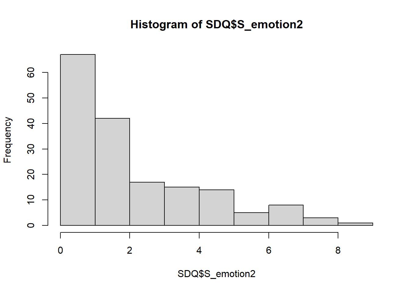
##    vars   n mean   sd median trimmed  mad min max range skew kurtosis   se
## X1    1 172 2.41 2.14      2    2.14 1.48   0   9     9 0.91     0.11 0.16
The histogram and the descriptive statistics for Time 2 look similar to Time 1. There is still a floor effect, with many pupils not endorsing any symptoms.
Q5. 13 children (or 5.7%) can be classified Borderline. You can look up the count for Borderline score 6 in the output of the basic table() function. Alternatively, you can call:
##
## FALSE  TRUE
## 215 13Importantly, you have to use == when describing the equality condition, because the use of = in R is reserved to assigning a value to an object.
Q6. For “Abnormal”, you can ask to tabulate all scores greater than 6. To calculate proportion, divide by N=228. This gives 20/228 = 0.88 or 8.8%.
##
## FALSE  TRUE
##   208    20
Q7.
Q8.
# reverse code
R_conduct2 <- reverse.code(keys=c(1,-1,1,1,1), SDQ[items_conduct2])
# check the reverse coded items
head(R_conduct2)
## tantrum2 obeys2- fights2 lies2 steals2
## [1,] 0 0 0 1 0
## [2,] 1 1 0 0 0
## [3,] 2 0 0 0 0
## [4,] 0 1 0 0 0
## [5,] NA NA NA NA NA
## [6,] 0 0 0 0 0## tantrum2 obeys2 fights2 lies2 steals2
## 1 0 2 0 1 0
## 2 1 1 0 0 0
## 3 2 2 0 0 0
## 4 0 1 0 0 0
## 5 NA NA NA NA NA
## 6 0 2 0 0 0Q9.
If you call SDQ$S_conduct2, you will see that there are many cases with missing score, labelled NaN. This is because the scale score cannot be computed for those pupils who had ALL responses missing at time 2.