Exercise 10 EFA of ability subtest scores
| Data file | Thurstone.csv |
| R package | psych |
10.1 Objectives
In this exercise, you will explore the factor structure of an ability test battery by analyzing observed correlations of its subtest scores.
10.2 Study of “primary mental abilities” by Louis Thurstone
This is a classic study of “primary mental abilities” by Louis Thurstone (1947). Thurstone analysed 9 subtests, each measuring some specific mental ability with several tasks. The 9 subtests were designed to measure 3 broader mental abilities, namely:
| Verbal Ability | Word Fluency | Reasoning Ability |
|---|---|---|
| 1. sentences | 4. first letters | 7. letter series |
| 2. vocabulary | 5. four-letter words | 8. pedigrees |
| 3. sentence completion | 6. suffixes | 9. letter grouping |
Each subtest was scored as a number of correctly completed tasks, and the scores on each of the 9 subtests can be considered continuous.
We will work with the published correlations between the 9 subtests, based on N=215 subjects. Despite having no access to the actual subject scores, the correlation matrix is all you need to run EFA.
10.3 Worked Example - EFA of Thurstone’s primary ability data
To complete this exercise, you need to repeat the analysis from a worked example below, and answer some questions.
Step 1. Importing and examining observed correlations
The data (subscale correlations) are stored in a comma-separated (.csv) file Thurstone.csv. Download this file and save it in a new folder. In RStudio, create a new project in the folder you have just created.
You can preview the file by clicking on Thurstone.csv in the Files tab in RStudio, and selecting View File. This will not import the data yet, just open the actual .csv file. You will see that the first row contains the subscale names - “s1”, “s2”, “s3”, etc., and the first entry in each row is again the facet names. To import this correlation matrix into RStudio preserving all these facet names for each row and each column, we will use function read.csv(). We will say that we have headers (header=TRUE), and that the row names are contained in the first column (row.names=1).
A new object Thurstone should appear in the Environment tab. Examine the object by either pressing on it, or calling function View().
You will see that it is a correlation matrix, with values 1 on the diagonal, and moderate to large positive values off the diagonal. This is typical for ability tests – they tend to correlate positively with each other.
Step 2. Examining suitability of data for factor analysis
First, load the package psych to enable access to its functionality. Conveniently, most functions in this package easily accommodate analysis with correlation matrices as well as with raw data.
##
## Attaching package: 'psych'
## The following object is masked _by_ '.GlobalEnv':
##
## ThurstoneBefore you start EFA, request the Kaiser-Meyer-Olkin (KMO) index – the measure of sampling adequacy (MSA):
## Kaiser-Meyer-Olkin factor adequacy
## Call: KMO(r = Thurstone)
## Overall MSA =  0.88
## MSA for each item =
##   s1   s2   s3   s4   s5   s6   s7   s8   s9
## 0.86 0.86 0.90 0.86 0.88 0.92 0.85 0.93 0.87
QUESTION 1. What is the overall measure of sampling adequacy (MSA)? Interpret this result.
Step 3. Determining the number of factors
In this case, we have a prior hypothesis that 3 broad domains of ability are underlying the 9 subtests. We begin the analysis with function fa.parallel() to produce a scree plot for the observed data, and compare it to that of a random (i.e. uncorrelated) data matrix of the same size. In addition to the actual data (our correlation matrix, Thurstone), we need to supply the sample size (n.obs=215) to enable simulation of random data, because from the correlation matrix alone it is impossible to know how big the sample was. We will keep the default estimation method (fm="minres"). We will display eigenvalues for both - principal components and factors (fa="both").
## Warning in fa.stats(r = r, f = f, phi = phi, n.obs = n.obs, np.obs = np.obs, :
## The estimated weights for the factor scores are probably incorrect.  Try a
## different factor score estimation method.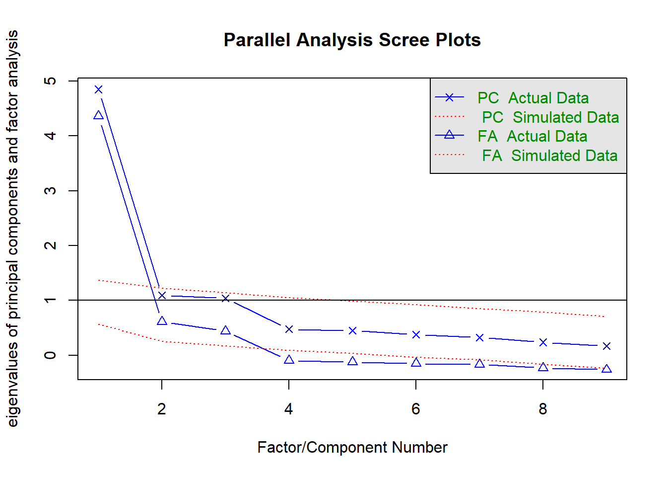
## Parallel analysis suggests that the number of factors = 3 and the number of components = 1Remember that when interpreting the scree plot, you retain only the factors on the blue (real data) scree plot that are ABOVE the red (simulated random data) plot, in which we know there is no common variance, only random variance, i.e. “scree” (rubble).
QUESTION 2. Examine the Scree plot. Does it support the hypothesis that 3 factors underlie the data? Why? Does your conclusion correspond to the text output of the parallel analysis function?
Step 4. Fitting an exploratory 1-factor model and assessing the model fit
We begin by fitting a single-factor model, which would correspond to a hypothesis that only one factor (presumably general mental ability) is needed to explain the pattern of correlations between 9 subtests. We will use function fa(), which has the following general form
fa(r, nfactors=1, n.obs = NA, rotate="oblimin", fm="minres" …),
and requires data (argument r), and the number of observations if the data is a correlation matrix (n.obs). Other arguments have defaults, which we are happy with for the first analysis.
Specifying all necessary arguments, test the hypothesized 1-factor model:
# fit 1-factor model
fit1 <- fa(Thurstone, nfactors=1, n.obs=215)
# print short summary with model fit
summary.psych(fit1)
##
## Factor analysis with Call: fa(r = Thurstone, nfactors = 1, n.obs = 215)
##
## Test of the hypothesis that 1 factor is sufficient.
## The degrees of freedom for the model is 27 and the objective function was 1.23
## The number of observations was 215 with Chi Square = 257.68 with prob < 1.7e-39
##
## The root mean square of the residuals (RMSA) is 0.1
## The df corrected root mean square of the residuals is 0.12
##
## Tucker Lewis Index of factoring reliability = 0.708
## RMSEA index = 0.199 and the 10 % confidence intervals are 0.178 0.222
## BIC = 112.67From the summary output, we find that Chi Square = 257.68 (df=27) with prob < 1.7e-39 - a highly significant result. According to the chi-square test, we have to reject the model. We also find that the root mean square of the residuals (RMSR) is 0.1. This is unacceptably high.
Next, let’s examine the model residuals, which are direct measures of model (mis)fit.
##    s1    s2    s3    s4    s5    s6    s7    s8    s9
## s1    NA
## s2  0.16    NA
## s3  0.14  0.13    NA
## s4 -0.11 -0.07 -0.07    NA
## s5 -0.10 -0.08 -0.09  0.23    NA
## s6 -0.05 -0.02 -0.04  0.18  0.14    NA
## s7 -0.05 -0.08 -0.08 -0.03  0.00 -0.09    NA
## s8  0.01 -0.01  0.02 -0.09 -0.07 -0.08  0.15    NA
## s9 -0.09 -0.12 -0.09  0.03  0.06 -0.03  0.24  0.07    NA
You can see that the residuals are mostly close to zero except those within clusters s1-s3, s4-s6, and s7-s9, where residuals mostly above 0.1 and as high as 0.24. Evidently, one factor cannot quite explain the dependencies of subtests within these clusters.
We conclude that the 1-factor model is not adequate for these data.
Step 5. Fitting an exploratory 3-factor models and assessing the model fit
Now let’s fit a 3-factor model to these data:
## Loading required namespace: GPArotation##
## Factor analysis with Call: fa(r = Thurstone, nfactors = 3, n.obs = 215)
##
## Test of the hypothesis that 3 factors are sufficient.
## The degrees of freedom for the model is 12 and the objective function was 0.01
## The number of observations was 215 with Chi Square = 3.01 with prob < 1
##
## The root mean square of the residuals (RMSA) is 0.01
## The df corrected root mean square of the residuals is 0.01
##
## Tucker Lewis Index of factoring reliability = 1.026
## RMSEA index = 0 and the 10 % confidence intervals are 0 0
## BIC = -61.44
## With factor correlations of
## MR1 MR2 MR3
## MR1 1.00 0.59 0.53
## MR2 0.59 1.00 0.52
## MR3 0.53 0.52 1.00QUESTION 3. What is the chi square statistic, and p value, for the tested 3-factor model? Would you retain or reject this model based on the chi-square test? Why?
QUESTION 4. Find and interpret the RMSR in the output.
Examine the 3-factor model residuals.
##    s1    s2    s3    s4    s5    s6    s7    s8    s9
## s1    NA
## s2  0.01    NA
## s3  0.00 -0.01    NA
## s4 -0.01  0.00  0.01    NA
## s5  0.01  0.00  0.00  0.00    NA
## s6  0.00  0.00  0.00  0.00  0.00    NA
## s7  0.00  0.01 -0.01  0.01 -0.01  0.00    NA
## s8 -0.01  0.00  0.02  0.00  0.00  0.01  0.00    NA
## s9  0.01 -0.01  0.00  0.00  0.01  0.00  0.00  0.00    NA
QUESTION 5. Examine the residual correlations. What can you say about them? Are there any non-trivial residuals (greater than 0.1 in absolute value)?
Step 6. Interpreting the 3-factor obliquely rotated solution
We will now interpret the 3-factor solution, which was rotated obliquely (by default, rotate="oblimin" is used in fa() function).
##
## Loadings:
##    MR1    MR2    MR3
## s1  0.901
## s2  0.890
## s3  0.838
## s4         0.853
## s5         0.747  0.104
## s6  0.180  0.626
## s7                0.842
## s8  0.382         0.463
## s9         0.212  0.627
##
##                  MR1   MR2   MR3
## SS loadings    2.489 1.732 1.337
## Proportion Var 0.277 0.192 0.149
## Cumulative Var 0.277 0.469 0.617
QUESTION 6. Examine the standardized factor loadings (pattern matrix), and name the factors you obtained based on which subtests load on them.
Examine the factor loading matrix again, this time looking for cross-loading facets (facets with loadings greater than 0.32 on factor(s) other than its own). Note that in the above output, loadings under 0.1 are suppressed by default. I use a 0.32 cut-off for non-trivial loadings since this translates into 10% of variance shared with the factor in an orthogonal solution. This value is quite arbitrary, and many use 0.3 instead.
QUESTION 7. Are there any non-trivial cross-loadings?
We now ask for “Phi” - the correlation matrix of latent factors. These correlations are model-based; that is, they are estimated within the model, as one of parameters. These correlations are between the latent factors (NOT their imperfect measurements, e.g. sum scores), and therefore they are the closest you can get to estimating how the actual ability domains are correlated in the population.
##           MR1       MR2       MR3
## MR1 1.0000000 0.5926277 0.5334434
## MR2 0.5926277 1.0000000 0.5151336
## MR3 0.5334434 0.5151336 1.0000000
QUESTION 8. Interpret the factor correlation matrix.
Step 7. Saving your work
After you finished work with this exercise, save your R script by pressing the Save icon in the script window. To keep all the created objects (such as FA_neo), which might be useful when revisiting this exercise, save your entire work space. To do that, when closing the project by pressing File / Close project, make sure you select Save when prompted to save your “Workspace image”.
10.4 Solutions
Q1. MSA = 0.88. According to Kaiser’s guidelines, the data are “meritorious” (i.e. very much suitable for factor analysis). Refer to Exercise 7 to remind yourself of this index and its interpretation.
Q2. The scree plot has a very steep drop from the first factor to the second, and then a slightly ambiguous “step” formed from the 2nd and the 3rd factors. The 2nd factor could already be considered part of “scree” (rubble), and Parallel Analysis based on PC (principal components) eigenvalues agrees with this judgement. Alternatively, the 2nd and 3rd factors could be considered parts of the hard rock and the “scree” beginnig with the 4th factor. Parallel Analysis based on FA (factor analysis) eigenvalues agrees with this alternative judgement. So, at this point we have an ambiguous result about the number of factors.
Q3. Chi-square=3.01 (df=12) with prob<1. Clearly, we cannot reject the model because the test is insignificant. To obtain the exact p-value, use
## [1] 0.9955007Q4. The root mean square of the residuals (RMSA) is 0.01
This is a very small value, indicating excellent fit.
Q5. The residual correlations are all very close to 0. There are no residuals greater than 0.1 in absolute value.
Q6. This obliquely rotated solution complies to the hypothesized structure and is easy to interpret. Factor 1 is comprised from subtests s1-s3. Factor 2 is comprised from subtests s4-s6. Factor 3 is comprised from subtests s7-s9. The factors can be labelled according to the prior hypothesis: Verbal Ability, Word Fluency and Reasoning Ability, and these are 3 correlated domains of ability.
Q7. Yes, subtest s8 “Pedigrees” cross-loads on F1 (loading = 0.382) as well as on its own domain F3 (loading = 0.463). We can interpret this result as that both Verbal Ability and Reasoning Ability are needed to complete this subtest.
Q8. All correlations between domains are positive and large (just over 0.5), which is to be expected from measures of ability.