Exercise 19 Fitting an autoregressive model to longitudinal test measurements
| Data file | WISC.RData |
| R package | lavaan |
19.1 Objectives
In this exercise, you will fit a special type of path analysis model - an autoregressive model. Such models involve repeated (observed) measurements over several time points, and each subsequent measurement is regressed on the previous one, hence the name. The only latent variables in these models are regression residuals; there are no common factors or errors of measurement. This exercise will demonstrate one of the weaknesses of Path Analysis, specifically, why it is important to model the measurement error for unreliable measures.
19.2 Study of longitudinal stability of ability test score across 4 time points
Data for this exercise is taken from a study by Osborne and Suddick (1972). In this study, N=204 children took the Wechsler Intelligence Test for Children (WISC) at ages 6, 7, 9 and 11. There are two subtests - Verbal and Non-verbal reasoning.
Scores on both tests were recorded for each child at each time point, resulting in 4 variables for the Verbal test (V1, V2, V3, V4) and 4 variables for the Non-verbal test (N1, N2, N3, N4).
In terms of data, we only have summary statistics - means, Standard Deviations and correlations of all the observed variables - which were reported in the article. As you can see in Figure 19.1 below, the mean of Verbal test increases as the children get older, and so does the mean of Non-verbal test. The Standard Deviations also increase, suggesting the increasing spread of scores over time. However, the test scores of the same kind correlate strongly, suggesting that there is certain stability to rank ordering of children; so that despite everyone improving their scores, the children doing best at Time 1 still tend to do better at Time 2, 3 and 4.
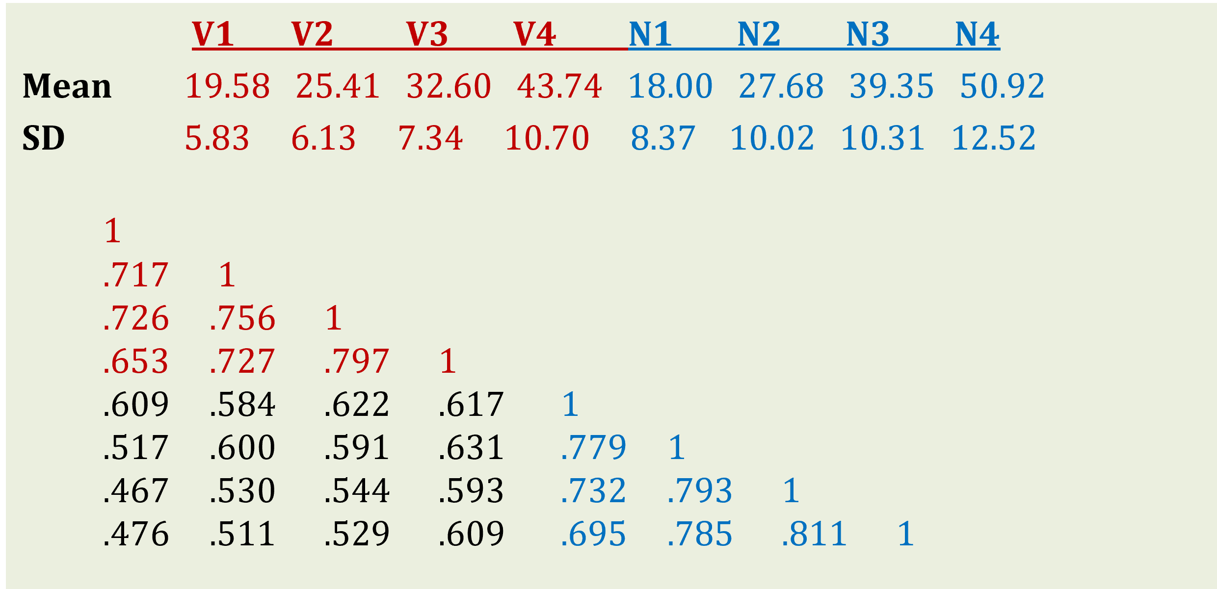
Figure 19.1: Descriptive statistics for WISC subtests
19.3 Worked Example - Testing an autoregressive model for WISC Verbal subtest
To complete this exercise, you need to repeat the analysis of Verbal subtests from a worked example below, and answer some questions. Once you are confident, you can repeat the analyses of Non-verbal subtests independently.
Step 1. Reading and examining data
The summary statistics are stored in the file WISC.RData. Download this file and save it in a new folder (e.g. “Autoregressive model of WISC data”). In RStudio, create a new project in the folder you have just created. Create a new R script, where you will be writing all your commands.
If you want to analyse the data straight away, you can simply load the prepared data into the environment:
Step 2 (Optional). Creating data objects for given means, SDs and correlations
Alternatively, as an exercise, you may follow me in creating the data objects from scratch using the descriptive statistics given in Figure 19.1.
WISC.mean <- c(19.58,25.41,32.60,43.74,18.00,27.68,39.35,50.92)

WISC.SD <- c(5.83,6.13,7.34,10.70,8.37,10.02,10.31,12.52)

# assign variable names
varnames = c("V1","V2","V3","V4","N1","N2","N3","N4")

# create a lower diagonal correlation matrix, with variable names
library(sem)
WISC.corr <- readMoments(diag=FALSE, names=varnames,
        text="
       .717
       .726 .756
       .653 .727 .797
       .609 .584 .622 .617
       .517 .600 .591 .631 .779
       .467 .530 .544 .593 .732 .793
       .476 .511 .529 .609 .695 .785 .811
")

# fill the upper triangle part with transposed values from the lower diagonal part
WISC.corr[upper.tri(WISC.corr)] <- t(WISC.corr)[upper.tri(WISC.corr)]

# save your objects to use them next time
save(WISC.mean, WISC.SD, WISC.corr, file='WISC.RData')
You should now see objects - WISC.mean, WISC.SD and WISC.corr in your Environment tab. Examine the objects by either clicking on them or passing them to the View() function, for example View(WISC.corr). You should see that WISC.corr is indeed a full correlation matrix, with values 1 on the diagonal.
Before we proceed to fitting a path model, however, we need to produce a covariance matrix for WISC data, because model fitting functions in lavaan work with covariance matrices. Of course you can supply a correlation matrix, but then you will lose the original measurement scale of your variables and essentially standardize them. I would like to keep the scale of WISC tests, and get unstandardized parameters. Thankfully, it is easy to produce a covariance matrix from the WISC correlation matrix and SDs. Since cov(X,Y) is the product of corr(X,Y), SD(X) and SD(Y), we can write:
Step 3. Specifying and fitting the model
Before you start modelling, load the package lavaan:
We will fit the following auto-regressive path model, for now without means (you can bring the means in as an optional challenge later).
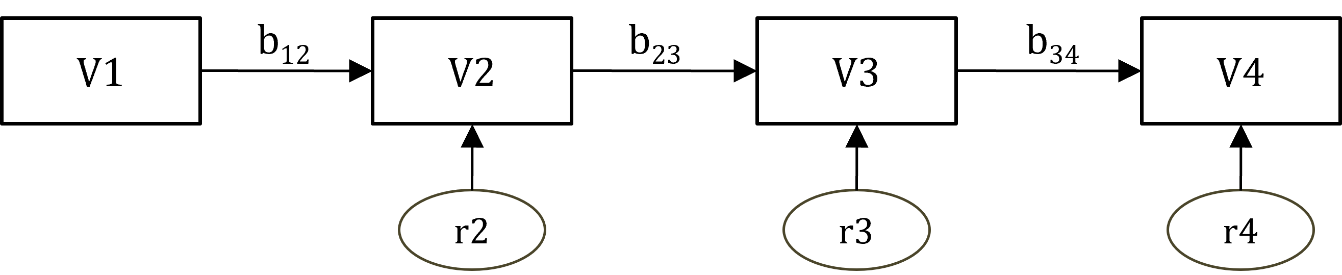
Figure 19.2: Autoregressive model for WISC Verbal subtest.
Coding this model using the lavaan syntax conventions is simple. You simply need to describe all the regression relationships in Figure 19.2. Let’s work from left to right of the diagram:
• V2 is regressed on V1 (residual for V2 is assumed)
• V3 is regressed on V2 (residual for V3 is assumed)
• V4 is regressed on V3 (residual for V4 is assumed)
That’s it. Try to write the respective statements using the shorthand symbol ~ for is regressed on. You should obtain something similar to this (I called my model V.auto, but you can call it whatever you like):
To fit this path model, we need function sem(). We need to pass to it: the model (model=V.auto, or simply V.auto if you put this argument first), and the data. However, the argument data is reserved for raw data (subjects by variables), but our data is the covariance matrix! So, we need to pass our matrix to the argument sample.cov, which is reserved for sample covariance matrices. We also need to pass the number of observations (sample.nobs = 204), because the covariance matrix does not provide this information.
Step 4. Assessing Goodness of Fit with global indices and residuals
To get access to model fitting results stored in object fit, request the extended output including fit measures and standardized parameter estimates:
## lavaan 0.6-19 ended normally after 1 iteration
##
##   Estimator                                         ML
##   Optimization method                           NLMINB
##   Number of model parameters                         6
##
##   Number of observations                           204
##
## Model Test User Model:
##
##   Test statistic                                58.473
##   Degrees of freedom                                 3
##   P-value (Chi-square)                           0.000
##
## Model Test Baseline Model:
##
##   Test statistic                               584.326
##   Degrees of freedom                                 6
##   P-value                                        0.000
##
## User Model versus Baseline Model:
##
##   Comparative Fit Index (CFI)                    0.904
##   Tucker-Lewis Index (TLI)                       0.808
##
## Loglikelihood and Information Criteria:
##
##   Loglikelihood user model (H0)              -1864.023
##   Loglikelihood unrestricted model (H1)      -1834.786
##
##   Akaike (AIC)                                3740.046
##   Bayesian (BIC)                              3759.955
##   Sample-size adjusted Bayesian (SABIC)       3740.945
##
## Root Mean Square Error of Approximation:
##
##   RMSEA                                          0.301
##   90 Percent confidence interval - lower         0.237
##   90 Percent confidence interval - upper         0.371
##   P-value H_0: RMSEA <= 0.050                    0.000
##   P-value H_0: RMSEA >= 0.080                    1.000
##
## Standardized Root Mean Square Residual:
##
##   SRMR                                           0.099
##
## Parameter Estimates:
##
##   Standard errors                             Standard
##   Information                                 Expected
##   Information saturated (h1) model          Structured
##
## Regressions:
##                    Estimate  Std.Err  z-value  P(>|z|)   Std.lv  Std.all
##   V2 ~
##     V1                0.754    0.051   14.691    0.000    0.754    0.717
##   V3 ~
##     V2                0.905    0.055   16.496    0.000    0.905    0.756
##   V4 ~
##     V3                1.162    0.062   18.847    0.000    1.162    0.797
##
## Variances:
##                    Estimate  Std.Err  z-value  P(>|z|)   Std.lv  Std.all
##    .V2               18.170    1.799   10.100    0.000   18.170    0.486
##    .V3               22.971    2.274   10.100    0.000   22.971    0.428
##    .V4               41.560    4.115   10.100    0.000   41.560    0.365
Examine the output, starting with parameter estimates. Look at column Std.all in the output, where parameters are based on all variables being standardized.
QUESTION 1. What is the standardized effect of V1 on V2? Can you relate this value to any of the observed sample moments? What about the standardized effects of V2 on V3, and V3 on V4?
Now carry out an assessment of the model’s goodness of fit, and try to answer the following questions.
QUESTION 2. How many parameters are there to estimate? How many known pieces of information (sample moments) are there in the data? What are the degrees of freedom and how are they calculated? [HINT. Remember that we are not interested in means here, only in covariance structure].
QUESTION 3. Interpret the chi-square. Do you retain or reject the model?
As I explained in Exercise 18, McDonald (1999) argued against the use of global fit indices such as RMSEA and CFI for path models and advocated for looking at the actual discrepancies [residuals]. To obtain residuals in the metric of correlation (differences between observed correlations and correlations ‘reproduced’ by the model), request this additional output:
## $type
## [1] "cor.bollen"
##
## $cov
##       V2    V3    V4    V1
## V2 0.000
## V3 0.000 0.000
## V4 0.124 0.000 0.000
## V1 0.000 0.184 0.221 0.000
Thinking of residuals as differences between 2 sets of correlations, we can easily interpret them. We usually interpret a correlation of 0.1 as small; and correlations below 0.1 trivial. Using this logic, we can see that all non-zero residuals (residuals for all relationships constrained by the model) are above 0.1 and cannot be ignored. These are residuals pertaining to relationships between non-adjacent time points - V1 and V3, V2 and V4 , and V1 and V4.
Step 5. Interpretation and critical appraisal of model results. The importance of accounting for measurement error.
What do these results mean? Shall we conclude that the model requires direct effects for non-adjacent measures, for example a direct path from V1 (verbal score at age 6) to V3 (score at age 9)?
A predictor is said to have a “sleeper” effect on a distal outcome if it influenced it not only indirectly through the more proximal outcome, but directly too. The unexplained relationships between distal points showing up in large residuals seem to suggest that we have such “sleeper” effects. For example, some variance in verbal score at age 9 that could not be explained by verbal score at age 7 could, however, be explained by the verbal score at age 6. It appears that some of the effect from age 6 was “sleeping” until age 9 when it resurfaced again.
Here we need to pause and look at the correlation structure implied by the autoregressive model and compare it with the correlations observed in this study.
If indeed the autoregressive relationships held, then any regression path is the product of the paths it consists of, for example:
b13 = b12 * b23.The standardized direct paths b12 and b23, as we worked out in Question 1, are equal to observed correlations between adjacent measures V1 and V2, and V2 and V3, respectively. But according to our data, b13 (0.726) is much larger than the product of b12 (0.717) and b23 (0.756), which should be 0.542. Our observed correlations fail to reduce to the extent the autoregressive model predicts.
To summarise, the autoregressive model predicts that the standardized indirect effect should get smaller the more distal the outcome is. But our data does not support this prediction. This finding is typical for the data of this kind. And the reason for it is not necessarily in the existence of “sleeper” effects, but could be often attributed to the failure to account for the error of measurement.
As you know, many psychological constructs such as “verbal reasoning” are not measured perfectly. According to the Classical Test Theory, variance in the observed measure (Y) is due to the ‘true’ score (T) and the measurement error (E):
var(Y) = var(T) + var(E)However, because the measurement errors are assumed uncorrelated, covariance of two measures Y1 and Y2 is due to ‘true’ scores only:
cov(Y1, Y2) = cov(T1, T2)Therefore, the error “contaminates” variances but not covariances. In the correlation matrix then, the off-diagonal elements reflect the relationships between the ‘true’ (standardized) scores, but the diagonal reflects the ‘true’ (standardized) score variances plus the measurement errors! So, the correlation matrix does NOT reflect correlations of ‘true’ scores. Instead, it reflects covariances of ‘true’ scores with variances smaller than 1. The actual correlations of ‘true’ scores could be estimated if we knew their variances. In Classical Test Theory, score reliability is defined as the proportion of variance in he observed score due to ‘true’ score. So, knowing and accounting for the score reliability would enable us to obtain correct estimates of the ‘true’ score correlations, and fit an autoregressive model to those estimates.
To conclude, it is important to appreciate limitations of path analysis. Path analysis deals with observed variables, and it assumes that these variables are measured without error. This assumption is almost always violated in psychological measurement. Test scores are not 100% reliable, and WISC scores in this data analysis example are no exception. Every time we deal with imperfect measures, we will encounter similar problems. The lower the reliability of our observed variables, the greater the problems might be. These need to be understood to draw correct conclusions from analysis.
To address this limitation, we need to account for the error of measurement. Models with measurement parts (where latent traits are indicated by observed variables) and structural parts (where we explore relationships between latent constructs - ‘true’ scores - rather than their imperfect measures) will be a way of dealing with unreliable data. I will provide such a full structural model for WISC data in Exercise 20.
Step 6. Saving your work
After you finished work with this exercise, save your R script with a meaningful name, for example “Autoregressive model of WISC”. To keep all of the created objects, which might be useful when revisiting this exercise, save your entire ‘work space’ when closing the project. Press File / Close project, and select “Save” when prompted to save your ‘Workspace image’.
19.4 Further practice - Path analysis of WISC Non-verbal scores
To practice further, fit an autoregressive path model to the WISC Non-verbal scores, and interpret the results.
19.5 Solutions
Q1. The standardized regression path are as follows
               Std.all
V2 ~  V1         0.717
V3 ~  V2         0.756
V4 ~  V3         0.797
These are equal to the observed correlations between V1 and V2, V2 and V3, and V3 and V4, respectively.
Q2. Let’s first calculate sample moments, which is the number of observed variances and covariances. There are 4 observed variables, therefore 4x(4+1)/2 = 10 moments in total (made up from 4 variances and 6 covariances).
The output prints that the “Number of model parameters” is 6. You can work out what these are just by looking at the diagram, or by counting the number of ‘Parameter estimates’ printed in the output. The best way to practice is to have a go just looking at the diagram, and then check with the output.
There are 3 regression paths (arrows on diagram) to estimate. There are also 3 paths from residuals to the observed variables, but they are fixed to 1 for setting the scale of residuals and therefore are not estimated. There are also variances of regression residuals. So far, this makes 3+3=6 parameters. But, there is actually one more parameter that lavaan does not print - the variance of independent variable V1. It is of course just the variance that we we already know from sample statistics, nevertheless, it is a model parameter (although trivial). [If you want the variance of V1 printed in the output, add the reference to it explicitly: V1 ~~ V1 ]
Then, the degrees of freedom is 3 (as lavvan rightly tells you), made up from 10(moments) – 7(parameters) = 3(df).
Q3. The chi-square test (Chi-square = 58.473, Degrees of freedom = 3, P-value < .001) suggests rejecting the model because the test is significant (p-value is very low). In this case, we cannot “blame” the poor chi-square result on the large sample size (N=204 is not that large).