Exercise 23 Testing for measurement invariance across sexes in a multiple-group setting
| Data file | HolzingerSwineford1939 |
| R package | lavaan, psych |
23.1 Objectives
The objective of this exercise is to fit a measurement model to two groups of participants using the multiple-group features of package lavaan. In particular, you will estimate means and variances of latent constructs in two groups, implementing measurement invariance constraints.
23.2 Study of structure of mental abilities
Holzinger and Swineford (1939) administered several mental ability tests to seventh and eighth-grade students in two Chicago schools. In the present example, we use scores obtained from 73 girls and 72 boys from the Grant-White school (Joreskog, 1969). Variables that we need for this exercise:
sex (1=boy, 2=girl)
school School (“Pasteur” or “Grant-White”)
x1 Visual perception test
x2 Spatial visualization test
x3 Spatial orientation test
x4 Paragraph comprehension test
x5 Sentence completion test
x6 Word meaning test
23.3 Worked Example - Comparing structure of mental abilities between sexes
To complete this exercise, you need to repeat the analysis from a worked example below, and answer some questions.
Step 1. Reading and examining data
The Holzinger-Swineford data set is included in package lavaan, so you do not need to download it separately.
Open RStudio, and create a new project, associating it with a new folder or perhaps with a folder where you downloaded this Workshop instruction.
Create a new R script. In the script, load the lavaan package, and then load the data set using the function data(). This function loads data included within packages.
A new object HolzingerSwineford1939 should appear in your Environment tab. Press on this object and the data set should open in its own tab. Examine it carefully, and scroll all the way down. You should notice that the beginning of the data set is populated with children from school “Pasteur”, and the end with children from school “Grant-White”. The latter is the school we need for our analysis. So, let’s create a new object called sample with only children from school Grant-White included.
In the above, I used the format dataset[rows,columns] to select only rows (cases) for which school equals “Grant-White”, retaining all columns (variables). If you look at the data frame sample in the Environment tab, it includes only 145 children from the Grant-White school, while the original data set had 301 children.
Examine the object sample using function head(). You will see that the variable sex is populated with numbers 1 (for boys) and 2 (for girls). Because this variable will be the focus of our analysis, it would be nice to have labels attached to these values, so each group is clearly labelled in all outputs. To do this, we use R base function factor(), which encodes a vector of values into categories (note that this function has nothing to do with factor analysis!). We would like to encode levels c(1,2) as two nominal categories c("boy", "girl"):
# give value labels for sex variable
sample$sex <- factor(sample$sex,
                    levels = c(1,2),
                    labels = c("boy", "girl"))
Request head(sample) again. You will see that now, variable sex is populated with either “boy” or “girl”.
Next, let’s obtain and examine the means of the six tests (x1 to x6) for boys and girls. An easy way to do this is to use function describeBy() from package psych:
##
##  Descriptive statistics by group
## sex: 1
##        vars  n   mean    sd median trimmed   mad    min    max  range  skew
## id        1 72 279.18 46.38 281.00  279.90 66.72 201.00 351.00 150.00 -0.10
## sex       2 72   1.00  0.00   1.00    1.00  0.00   1.00   1.00   0.00   NaN
## ageyr     3 72  12.90  1.05  13.00   12.84  1.48  11.00  16.00   5.00  0.62
## agemo     4 72   5.19  3.37   5.00    5.12  4.45   0.00  11.00  11.00  0.12
## school    5 72   1.00  0.00   1.00    1.00  0.00   1.00   1.00   0.00   NaN
## grade     6 71   7.49  0.50   7.00    7.49  0.00   7.00   8.00   1.00  0.03
## x1        7 72   4.97  1.16   4.92    4.97  1.11   2.67   8.50   5.83  0.17
## x2        8 72   6.23  1.10   6.00    6.13  1.11   4.00   9.25   5.25  0.64
## x3        9 72   2.14  1.08   1.88    2.08  1.11   0.38   4.38   4.00  0.40
## x4       10 72   3.10  1.02   3.00    3.08  0.99   0.33   6.00   5.67  0.26
## x5       11 72   4.60  1.05   4.75    4.62  1.11   1.75   6.50   4.75 -0.17
## x6       12 72   2.36  1.08   2.29    2.27  1.06   0.57   5.57   5.00  0.85
## x7       13 72   3.85  1.02   3.72    3.82  1.06   1.87   6.48   4.61  0.25
## x8       14 72   5.60  1.22   5.55    5.51  1.11   3.60  10.00   6.40  0.87
## x9       15 72   5.30  0.93   5.25    5.30  1.01   3.28   7.39   4.11  0.05
##        kurtosis   se
## id        -1.38 5.47
## sex         NaN 0.00
## ageyr      0.55 0.12
## agemo     -1.22 0.40
## school      NaN 0.00
## grade     -2.03 0.06
## x1        -0.06 0.14
## x2        -0.10 0.13
## x3        -0.91 0.13
## x4         0.50 0.12
## x5        -0.44 0.12
## x6         0.65 0.13
## x7        -0.50 0.12
## x8         1.46 0.14
## x9        -0.70 0.11
## ------------------------------------------------------------
## sex: 2
##        vars  n   mean    sd median trimmed   mad    min    max  range  skew
## id        1 73 271.38 40.06 270.00  270.61 45.96 202.00 348.00 146.00  0.11
## sex       2 73   2.00  0.00   2.00    2.00  0.00   2.00   2.00   0.00   NaN
## ageyr     3 73  12.55  0.85  12.00   12.49  0.00  11.00  15.00   4.00  0.59
## agemo     4 73   5.49  3.61   5.00    5.49  4.45   0.00  11.00  11.00  0.00
## school    5 73   1.00  0.00   1.00    1.00  0.00   1.00   1.00   0.00   NaN
## grade     6 73   7.41  0.50   7.00    7.39  0.00   7.00   8.00   1.00  0.35
## x1        7 73   4.89  1.15   5.00    4.94  0.99   1.83   7.50   5.67 -0.40
## x2        8 73   6.17  1.13   6.25    6.15  1.11   2.25   9.25   7.00 -0.13
## x3        9 73   1.85  0.99   1.62    1.75  0.93   0.38   4.50   4.12  0.82
## x4       10 73   3.53  1.19   3.33    3.49  0.99   0.67   6.33   5.67  0.37
## x5       11 73   4.83  1.26   5.00    4.95  1.11   1.00   7.00   6.00 -0.82
## x6       12 73   2.57  1.19   2.29    2.51  1.06   0.29   5.86   5.57  0.56
## x7       13 73   3.99  1.05   4.00    3.97  1.10   1.30   6.30   5.00  0.06
## x8       14 73   5.38  0.84   5.50    5.41  0.74   3.05   7.15   4.10 -0.41
## x9       15 73   5.35  1.12   5.47    5.36  1.07   3.11   9.25   6.14  0.25
##        kurtosis   se
## id        -1.04 4.69
## sex         NaN 0.00
## ageyr     -0.18 0.10
## agemo     -1.28 0.42
## school      NaN 0.00
## grade     -1.90 0.06
## x1        -0.36 0.13
## x2         1.32 0.13
## x3         0.04 0.12
## x4        -0.31 0.14
## x5         0.44 0.15
## x6        -0.29 0.14
## x7        -0.38 0.12
## x8         0.08 0.10
## x9         0.69 0.13
QUESTION 1. Examine the means of the six test variables for boys and girls. Note the mean differences for x3 (spatial orientation), and all verbal tests (x4-x6). Who score higher on what tests?
Step 2. Fitting a baseline measurement model to two groups (boys and girls)
It is thought that performance on the first three tests (x1, x2 and x3) depends on a broader spatial ability, whereas performance on the other three tests (x4, x5 and x6) depends on a broader verbal ability. We will fit a confirmatory factor model with two factors – Spatial and Verbal, which are expected to correlate. We will scale the factors by adopting the unit of their first indicators (x1 for Spatial, and x4 for Verbal), which is the default in lavaan.
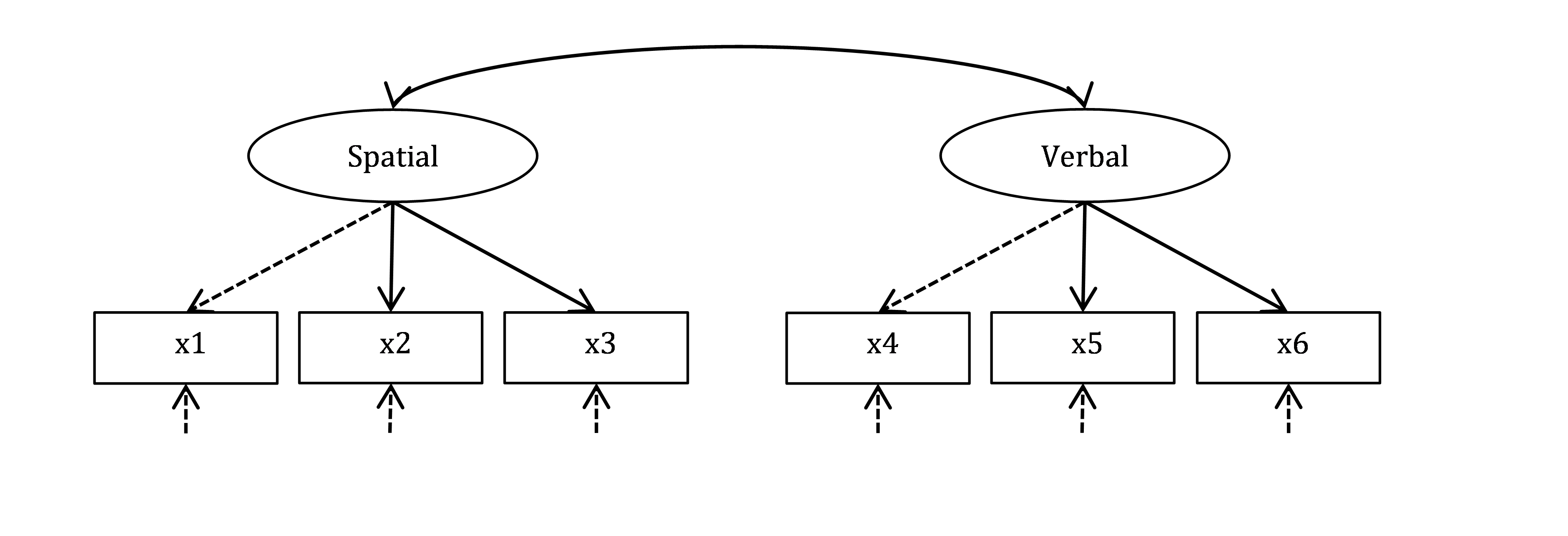
Figure 23.1: Measurement model for Holzinger and Swineford data.
OK, let’s first describe the measurement (confirmatory factor analysis, or CFA) model depicted in Figure 23.1. We will call it HS.model (HS stands for Holzinger-Swineford). You should be able to specify this model yourself by now, using the “measured by” (=~) syntax conventions:
Now we will fit the model using function cfa(). There is only one change from how we used this function before. This time, we want to perform a multiple-group analysis, and fit the model not to the whole sample of 145 children, but separately to two groups - 73 girls and 72 boys. In order to do this, we set sex as the grouping variable for analysis (group = "sex").
When we specify the grouping variable (group = "sex"), the data will be separated into two groups according to children sex, and the HS.model will be fitted to both groups without any parameter constraints. That is, all model parameters in each group will be freely estimated. This is called configural invariance, because the only thing in common between the groups is the configuration of the model (what variables indicate what factors).
NOTE that the default in multiple-group analysis is to include means/intercepts, so we do not need to specify this.
QUESTION 2. How many sample moments are there in the data? Why? {Hint. When counting sample moments, do not forget that we split the data into 2 groups, so observed means, variances and covariances are available for both groups}.
QUESTION 3. How many parameters does the baseline (configural) model estimate? What are they? {Hint. You can look up the total number of parameters in the output, but try to work out how these are made up. The output will help you, if you look in ‘Parameter Estimates’. Remember that values printed there are parameters.}
QUESTION 4. Interpret the chi-square, and SRMR. Do you retain or reject the baseline model?
Step 3. Fitting a full measurement invariance model to two groups
The baseline model does not allow us to compare the Spatial and Verbal factor scores between boys and girls, because each group has its own metric for these factors. For instance, origins of the factors are set to 0 in each group by default, so girls and boys form their own ‘norm’ groups. Girls can be compared with girls; boys with boys, but cross-comparison are not meaningful because the scale is “reset”. To compare the factor scores across groups properly, we need full measurement invariance. We want the factor loadings, intercepts and residual variances to be equal for every corresponding test across groups. They will be still estimable parameters, but instead of estimating two sets – for boys and for girls, we will estimate only one set for both groups.
This is very simple to do in lavaan. You do not need to adjust the model. You only need to tell the cfa() function which types of parameters you want to constrain equal across groups using argument group.equal. Because we want loadings, intercepts and residuals to be equal, we combine these parameter types into a vector using base R function c():
# Fitting Measurement Invariance model
fit.mi <- cfa(HS.model, data = sample, group = "sex",
           group.equal = c("loadings", "intercepts", "residuals"))

summary(fit.mi, fit.measures=TRUE)
## lavaan 0.6-19 ended normally after 44 iterations
##
## Estimator ML
## Optimization method NLMINB
## Number of model parameters 40
## Number of equality constraints 16
##
## Number of observations per group:
## boy 72
## girl 73
##
## Model Test User Model:
##
## Test statistic 27.482
## Degrees of freedom 30
## P-value (Chi-square) 0.598
## Test statistic for each group:
## boy 13.693
## girl 13.789
##
## Model Test Baseline Model:
##
## Test statistic 342.274
## Degrees of freedom 30
## P-value 0.000
##
## User Model versus Baseline Model:
##
## Comparative Fit Index (CFI) 1.000
## Tucker-Lewis Index (TLI) 1.008
##
## Loglikelihood and Information Criteria:
##
## Loglikelihood user model (H0) -1164.566
## Loglikelihood unrestricted model (H1) -1150.825
##
## Akaike (AIC) 2377.131
## Bayesian (BIC) 2448.573
## Sample-size adjusted Bayesian (SABIC) 2372.628
##
## Root Mean Square Error of Approximation:
##
## RMSEA 0.000
## 90 Percent confidence interval - lower 0.000
## 90 Percent confidence interval - upper 0.079
## P-value H_0: RMSEA <= 0.050 0.807
## P-value H_0: RMSEA >= 0.080 0.047
##
## Standardized Root Mean Square Residual:
##
## SRMR 0.058
##
## Parameter Estimates:
##
## Standard errors Standard
## Information Expected
## Information saturated (h1) model Structured
##
##
## Group 1 [boy]:
##
## Latent Variables:
## Estimate Std.Err z-value P(>|z|)
## Spatial =~
## x1 1.000
## x2 (.p2.) 0.813 0.173 4.699 0.000
## x3 (.p3.) 1.063 0.200 5.302 0.000
## Verbal =~
## x4 1.000
## x5 (.p5.) 0.963 0.084 11.442 0.000
## x6 (.p6.) 0.947 0.082 11.520 0.000
##
## Covariances:
## Estimate Std.Err z-value P(>|z|)
## Spatial ~~
## Verbal 0.387 0.116 3.329 0.001
##
## Intercepts:
## Estimate Std.Err z-value P(>|z|)
## .x1 (.16.) 5.021 0.118 42.462 0.000
## .x2 (.17.) 6.274 0.108 57.911 0.000
## .x3 (.18.) 2.092 0.113 18.468 0.000
## .x4 (.19.) 3.157 0.117 27.051 0.000
## .x5 (.20.) 4.558 0.118 38.678 0.000
## .x6 (.21.) 2.317 0.115 20.093 0.000
##
## Variances:
## Estimate Std.Err z-value P(>|z|)
## .x1 (.p7.) 0.799 0.128 6.223 0.000
## .x2 (.p8.) 0.883 0.123 7.209 0.000
## .x3 (.p9.) 0.487 0.110 4.439 0.000
## .x4 (.10.) 0.289 0.063 4.572 0.000
## .x5 (.11.) 0.443 0.073 6.094 0.000
## .x6 (.12.) 0.412 0.069 5.990 0.000
## Spatial 0.484 0.165 2.931 0.003
## Verbal 0.769 0.164 4.689 0.000
##
##
## Group 2 [girl]:
##
## Latent Variables:
## Estimate Std.Err z-value P(>|z|)
## Spatial =~
## x1 1.000
## x2 (.p2.) 0.813 0.173 4.699 0.000
## x3 (.p3.) 1.063 0.200 5.302 0.000
## Verbal =~
## x4 1.000
## x5 (.p5.) 0.963 0.084 11.442 0.000
## x6 (.p6.) 0.947 0.082 11.520 0.000
##
## Covariances:
## Estimate Std.Err z-value P(>|z|)
## Spatial ~~
## Verbal 0.395 0.134 2.956 0.003
##
## Intercepts:
## Estimate Std.Err z-value P(>|z|)
## .x1 (.16.) 5.021 0.118 42.462 0.000
## .x2 (.17.) 6.274 0.108 57.911 0.000
## .x3 (.18.) 2.092 0.113 18.468 0.000
## .x4 (.19.) 3.157 0.117 27.051 0.000
## .x5 (.20.) 4.558 0.118 38.678 0.000
## .x6 (.21.) 2.317 0.115 20.093 0.000
## Spatial -0.180 0.145 -1.245 0.213
## Verbal 0.318 0.172 1.847 0.065
##
## Variances:
## Estimate Std.Err z-value P(>|z|)
## .x1 (.p7.) 0.799 0.128 6.223 0.000
## .x2 (.p8.) 0.883 0.123 7.209 0.000
## .x3 (.p9.) 0.487 0.110 4.439 0.000
## .x4 (.10.) 0.289 0.063 4.572 0.000
## .x5 (.11.) 0.443 0.073 6.094 0.000
## .x6 (.12.) 0.412 0.069 5.990 0.000
## Spatial 0.538 0.180 2.989 0.003
## Verbal 1.114 0.227 4.917 0.000What you have just done is fitted a full measurement invariance model. The model tests the following combined hypothesis:
H1. The measure is fully invariant across groups. Factor loadings, intercepts and error variances for corresponding indicators are equal.
QUESTION 5. Interpret the chi-square and SRMR. Do we retain or reject the full measurement invariance model?
Now examine the output, focusing on ‘Parameter Estimates’. Note that all those measurement parameters that were supposed to be equal are indeed equal!
Here is a brief explanation of why the parameters are set the way they are. While we assume full measurement invariance (i.e. the tests function equally across groups), we do not have any particular reasons to assume that boys and girls should be equal to each other in terms of their latent factors – Spatial and Verbal. In fact, they might be different with respect to group means, variances and covariances. This is why the logical way of scaling the latent factors is setting their metric in the first group (say, boys), and carry over that metric to the second group (girls) via parameter constraints. The parameter constraints will ensure the scale of measurement does not change, and then the means, variances and covariances of the latent factors for girls can be freely estimated.
QUESTION 6. How many parameters does the measurement invariance model estimate? What are they? {Hint. Again, look up the total number of parameters in the output, and then try to work out how these are made up. The ‘Parameter Estimates’ output and the above explanation will help you.}
Now, examine and interpret the means, variances and covariances of Spatial and Verbal factors.
QUESTION 7. What are the means and variances of Spatial and Verbal for Girls? How do you interpret these values?
Step 4. Testing equality of means of latent factors
There are small differences between the means of Spatial and Verbal for boys and girls. It appears that girls are slightly worse than boys in spatial ability, but better in verbal ability. However, the means for girls were not significantly different from 0 at the 0.05 level, which could also lead us to conclude that they were not significantly different from boy’s means (see answer to Question 7 for explanation).
Let us test the hypothesis of equality of the means of Spatial and Verbal for girls and boys formally. All you need to do is to add one more group equality constraint, for the "means" of latent variables:
# Testing Equality of means of latent factors
fit.mi.e <- cfa(HS.model, data = sample, group = "sex",
   group.equal = c("loadings", "intercepts", "residuals", "means"))

summary(fit.mi.e, fit.measures=TRUE)
## lavaan 0.6-19 ended normally after 41 iterations
##
## Estimator ML
## Optimization method NLMINB
## Number of model parameters 38
## Number of equality constraints 16
##
## Number of observations per group:
## boy 72
## girl 73
##
## Model Test User Model:
##
## Test statistic 35.786
## Degrees of freedom 32
## P-value (Chi-square) 0.295
## Test statistic for each group:
## boy 17.258
## girl 18.528
##
## Model Test Baseline Model:
##
## Test statistic 342.274
## Degrees of freedom 30
## P-value 0.000
##
## User Model versus Baseline Model:
##
## Comparative Fit Index (CFI) 0.988
## Tucker-Lewis Index (TLI) 0.989
##
## Loglikelihood and Information Criteria:
##
## Loglikelihood user model (H0) -1168.718
## Loglikelihood unrestricted model (H1) -1150.825
##
## Akaike (AIC) 2381.435
## Bayesian (BIC) 2446.923
## Sample-size adjusted Bayesian (SABIC) 2377.308
##
## Root Mean Square Error of Approximation:
##
## RMSEA 0.040
## 90 Percent confidence interval - lower 0.000
## 90 Percent confidence interval - upper 0.099
## P-value H_0: RMSEA <= 0.050 0.555
## P-value H_0: RMSEA >= 0.080 0.158
##
## Standardized Root Mean Square Residual:
##
## SRMR 0.078
##
## Parameter Estimates:
##
## Standard errors Standard
## Information Expected
## Information saturated (h1) model Structured
##
##
## Group 1 [boy]:
##
## Latent Variables:
## Estimate Std.Err z-value P(>|z|)
## Spatial =~
## x1 1.000
## x2 (.p2.) 0.810 0.172 4.707 0.000
## x3 (.p3.) 1.012 0.195 5.185 0.000
## Verbal =~
## x4 1.000
## x5 (.p5.) 0.977 0.086 11.401 0.000
## x6 (.p6.) 0.960 0.084 11.480 0.000
##
## Covariances:
## Estimate Std.Err z-value P(>|z|)
## Spatial ~~
## Verbal 0.384 0.117 3.267 0.001
##
## Intercepts:
## Estimate Std.Err z-value P(>|z|)
## .x1 (.16.) 4.938 0.095 51.820 0.000
## .x2 (.17.) 6.207 0.092 67.524 0.000
## .x3 (.18.) 2.004 0.086 23.313 0.000
## .x4 (.19.) 3.277 0.092 35.697 0.000
## .x5 (.20.) 4.672 0.095 49.199 0.000
## .x6 (.21.) 2.430 0.093 26.199 0.000
##
## Variances:
## Estimate Std.Err z-value P(>|z|)
## .x1 (.p7.) 0.778 0.131 5.939 0.000
## .x2 (.p8.) 0.871 0.123 7.072 0.000
## .x3 (.p9.) 0.520 0.111 4.689 0.000
## .x4 (.10.) 0.306 0.064 4.758 0.000
## .x5 (.11.) 0.434 0.073 5.978 0.000
## .x6 (.12.) 0.403 0.069 5.858 0.000
## Spatial 0.504 0.172 2.934 0.003
## Verbal 0.770 0.165 4.662 0.000
##
##
## Group 2 [girl]:
##
## Latent Variables:
## Estimate Std.Err z-value P(>|z|)
## Spatial =~
## x1 1.000
## x2 (.p2.) 0.810 0.172 4.707 0.000
## x3 (.p3.) 1.012 0.195 5.185 0.000
## Verbal =~
## x4 1.000
## x5 (.p5.) 0.977 0.086 11.401 0.000
## x6 (.p6.) 0.960 0.084 11.480 0.000
##
## Covariances:
## Estimate Std.Err z-value P(>|z|)
## Spatial ~~
## Verbal 0.384 0.137 2.811 0.005
##
## Intercepts:
## Estimate Std.Err z-value P(>|z|)
## .x1 (.16.) 4.938 0.095 51.820 0.000
## .x2 (.17.) 6.207 0.092 67.524 0.000
## .x3 (.18.) 2.004 0.086 23.313 0.000
## .x4 (.19.) 3.277 0.092 35.697 0.000
## .x5 (.20.) 4.672 0.095 49.199 0.000
## .x6 (.21.) 2.430 0.093 26.199 0.000
##
## Variances:
## Estimate Std.Err z-value P(>|z|)
## .x1 (.p7.) 0.778 0.131 5.939 0.000
## .x2 (.p8.) 0.871 0.123 7.072 0.000
## .x3 (.p9.) 0.520 0.111 4.689 0.000
## .x4 (.10.) 0.306 0.064 4.758 0.000
## .x5 (.11.) 0.434 0.073 5.978 0.000
## .x6 (.12.) 0.403 0.069 5.858 0.000
## Spatial 0.578 0.192 3.012 0.003
## Verbal 1.134 0.232 4.888 0.000The resulting model tests the following combined hypothesis:
H1. The measure is fully invariant across groups. Factor loadings, intercepts and error variances for corresponding indicators are equal.
H2. The means of Spatial and Verbal factors are equal across groups.
The model with equality constraints on latent means (fit.mi.e) appears to fit well based on the chi-square test, and the SRMR=0.078 is just under the acceptable value of 0.08.
Next, we will formally compare two models – the measurement invariance model (fit.mi) and the measurement invariance model with equality constraints (fit.mi.e). It would be interesting to know if the two models are significantly different from each other.
Because the two models are nested (one is a special case of the other), you can conduct the chi-square difference test using the R base function anova(), which will compute the difference of the models’ chi-square statistics and the difference of their degrees of freedom, and print out the resulting p-value.
QUESTION 8. Conduct the chi-square difference test of models with and without the equality constraints as described above, and interpret the results. Are the models significantly different? Which model will you retain?
Step 5. Saving your work
After you finished work with this exercise, save your R script with a meaningful name, for example “Holzinger-Swineford 1939 analysis”.
To keep all of the created objects, which might be useful when revisiting this exercise, save your entire ‘work space’ when closing the project. Press File / Close project, and select Save when prompted to save your ‘Workspace image’.
23.4 Solutions
Q1. Boys scored higher than girls on x3, but girls scored higher than boys on all verbal tests (x4, x5 and x6).
Q2. As we model means/intercepts too, we need to include them in the counted sample moments. ‘Sample moments’ refers to the number of means, variances and covariances in the observed data. There are 6 observed variables, therefore 6 means, plus 6(6+1)/2=21 variances and covariances; 27 moments in total for each group. So we have 27*2=54 sample moments across both groups.
Q3. Baseline model estimates 38 parameters in total. Boys and girls groups estimate the same parameters (i.e. there are 19 parameters in each group). These are:
• 4 factor loadings (loadings for x1 and x4 are fixed to 1);
• 1 covariance of Spatial and Verbal factors;
• 6 intercepts of observed variables x1-x6;
• 6 residual variances of observed variables x1-x6;
• 2 variances (for Spatial and Verbal factors).
Q4. Chi-square for the baseline model is insignificant (chisq = 16.710; Degrees of freedom = 16; p = .405). The SMRR is 0.040 – nice and small.
A breakdown of the chi-square statistic by group is also provided, attributing 8.748 to boys, and 7.962 to girls (the chi-square statistic is additive, so these values add to the total chi-square statistic reported). The almost equal chi-square values for both groups (and the groups were of almost equal size) indicate similar fit of the baseline model in both groups. We conclude that the two-factor configural model is appropriate for boys and girls.
Q5. Chi-square for the measurement invariance model is again insignificant (chisq = 27.482, Degrees of freedom = 30, P-value = 0.598). The SMRR is 0.058 – small again. The almost equal chi-square values for both groups (boy chisq = 13.693, girl chisq = 13.789) indicate that the measurement invariance model is equally appropriate for boys and girls.
Q6. The output says that ‘Number of free parameters’ is 40, and ‘Number of equality constraints’ is 16. This means that 40-16=24 unique parameters are estimated:
• 4 factor loadings (note that these have labels and parameter values identical for boys and girls);
• 1 covariance of Spatial and Verbal for boys + 1 covariance for girls (note that these have no labels and the values are different in the output) ;
• 6 intercepts of observed variables x1-x6 (note that these have labels and parameter values identical for boys and girls);
• 2 means of Spatial and Verbal factors for girls (note that for boys, these means are set to 0);
• 6 residual variances of observed variables x1-x6 (note that these have labels and parameter values identical for boys and girls);
• 2 variances of Spatial and Verbal factors for boys + 2 variances for girls.
Q7. For Girls, the mean for Spatial is –0.180 (which appears lower than for Boys for whom the mean was fixed to 0), and the mean for Verbal is 0.318 (higher than for Boys for whom the mean was fixed to 0). Both means for girls are not significantly different from zero at the 0.05 level (look at their p-values).
Variances of the Spatial and Verbal factors are larger for girls (0.538; 1.114) than boys (0.484; 0.769). Girls appear to show more variability in their latent abilities than boys.
Q8. The model with additional constraints (fit.mi.e) has the Chi-square = 35.786; Degrees of freedom = 32. Testing the difference between this model and the previous model (fit.mi), we obtain Diff(Chi-square) = 35.786–27.482= 8.304 and Diff(DF) = 32–30 = 2.
Chi-square of 8.304 on 2 degrees of freedom is significant at the 0.05 level, with the p-value=0.016. Restricting the model with additional equality constraints resulted in significantly different (worse) fit. The fit is worse is because the chi-square is greater (and constraining some free parameters cannot make the fit better!). We conclude that the means for boys and girls on the Spatial and Verbal tests are significantly different, and that our measurement invariance model with free means is better than the model with means constrained equal.
You may wonder how the fit can be ‘significantly worse’ if it is still very good according to the chi-square test (the SRMR, not being a ‘significance’ measure but an ‘effect size’ measure picked up the worsening fit). Here the small sample works against us – there is not enough power to reject the ‘wrong’ model (it has too many parameters), but just enough power to detect the elements of the model that make a difference.