Exercise 8 Fitting a single-factor model to dichotomous questionnaire data
| Data file | EPQ_N_demo.txt |
| R package | psych |
8.1 Objectives
The objective of this exercise is to test homogeneity of a questionnaire compiled from dichotomous items, by fitting a single-factor model to tetrachoric correlations of the questionnaire items rather than product-moment (Pearson’s) correlations.
8.2 Worked Example - Testing homogeneity of EDQ Neuroticism scale
To complete this exercise, you need to repeat the analysis from a worked example below, and answer some questions.
This exercise makes use of the data we considered in Exercise 6. These data come from a a large cross-cultural study (Barrett, Petrides, Eysenck & Eysenck, 1998), with N = 1,381 participants who completed the Eysenck Personality Questionnaire (EPQ).
The focus of our analysis here will be the Neuroticism/Anxiety (N) scale, measured by 23 items with only two response options - either “YES” or “NO”, for example:
N_3     Does your mood often go up and down?
N_7     Do you ever feel "just miserable" for no reason?
N_12    Do you often worry about things you should not have done or said?
etc.
You can find the full list of EPQ Neuroticism items in Exercise 6. Please note that all items indicate “Neuroticism” rather than “Emotional Stability” (i.e. there are no counter-indicative items).
Step 1. Opening and examining the data
If you have already worked with this data set in Exercise 6, the simplest thing to do is to continue working within the project created back then. In RStudio, select File / Open Project and navigate to the folder and the project you created. You should see the data frame EPQ appearing in your Environment tab, together with other objects you created and saved.
If you have not completed Exercise 6 or have not saved your work, or simply want to start from scratch, download the data file EPQ_N_demo.txt into a new folder and follow instructions from Exercise 6 on creating a project and importing the data.
The object EPQ should appear on the Environment tab. Click on it and the data will be displayed on a separate tab. As you can see, there are 26 variables in this data frame, beginning with participant id, age and sex (0 = female; 1 = male). These demographic variables are followed by 23 item responses, which are either 0 (for “NO”) or 1 (for “YES”). There are also a few missing responses, marked with NA.
Step 2. Examining suitability of data for factor analysis
Now, load the package psych to enable access to its functionality:
Before starting factor analysis, check correlations between responses to the 23 items. Package psych has function lowerCor()that prints the correlation matrix in a compact format. Note that to refer to the 23 item responses only, you need to specify the columns where they are stored (from 4 to 26):
##      N_3  N_7  N_12 N_15 N_19 N_23 N_27 N_31 N_34 N_38 N_41
## N_3  1.00
## N_7  0.36 1.00
## N_12 0.26 0.28 1.00
## N_15 0.31 0.21 0.12 1.00
## N_19 0.33 0.30 0.32 0.18 1.00
## N_23 0.36 0.30 0.24 0.28 0.28 1.00
## N_27 0.28 0.28 0.31 0.24 0.32 0.29 1.00
## N_31 0.24 0.20 0.18 0.22 0.31 0.24 0.26 1.00
## N_34 0.30 0.33 0.34 0.20 0.41 0.32 0.36 0.45 1.00
## N_38 0.26 0.24 0.28 0.21 0.29 0.27 0.33 0.28 0.41 1.00
## N_41 0.23 0.21 0.16 0.29 0.27 0.26 0.23 0.43 0.35 0.27 1.00
## N_47 0.17 0.13 0.19 0.09 0.16 0.20 0.20 0.18 0.20 0.29 0.14
## N_54 0.20 0.19 0.11 0.20 0.15 0.16 0.15 0.20 0.18 0.16 0.21
## N_58 0.36 0.34 0.22 0.19 0.24 0.35 0.24 0.18 0.22 0.20 0.16
## N_62 0.26 0.23 0.14 0.23 0.20 0.29 0.20 0.20 0.23 0.19 0.24
## N_66 0.20 0.16 0.27 0.12 0.25 0.24 0.22 0.17 0.24 0.25 0.13
## N_68 0.22 0.29 0.15 0.19 0.22 0.21 0.22 0.14 0.21 0.19 0.15
## N_72 0.24 0.32 0.32 0.13 0.42 0.24 0.34 0.29 0.41 0.29 0.26
## N_75 0.26 0.29 0.21 0.25 0.31 0.27 0.25 0.53 0.38 0.28 0.40
## N_77 0.33 0.30 0.18 0.23 0.29 0.37 0.31 0.26 0.29 0.25 0.25
## N_80 0.23 0.23 0.27 0.10 0.56 0.19 0.29 0.28 0.35 0.24 0.25
## N_84 0.25 0.22 0.15 0.08 0.14 0.18 0.16 0.10 0.15 0.13 0.09
## N_88 0.19 0.17 0.12 0.12 0.19 0.17 0.13 0.05 0.17 0.15 0.11
##      N_47 N_54 N_58 N_62 N_66 N_68 N_72 N_75 N_77 N_80 N_84
## N_47 1.00
## N_54 0.09 1.00
## N_58 0.16 0.20 1.00
## N_62 0.07 0.16 0.20 1.00
## N_66 0.21 0.11 0.16 0.15 1.00
## N_68 0.05 0.17 0.21 0.24 0.14 1.00
## N_72 0.18 0.08 0.21 0.19 0.27 0.22 1.00
## N_75 0.19 0.25 0.24 0.23 0.19 0.16 0.30 1.00
## N_77 0.11 0.23 0.27 0.41 0.24 0.28 0.27 0.29 1.00
## N_80 0.11 0.13 0.18 0.14 0.25 0.21 0.40 0.30 0.26 1.00
## N_84 0.12 0.12 0.29 0.14 0.11 0.16 0.13 0.12 0.17 0.13 1.00
## N_88 0.09 0.07 0.16 0.07 0.12 0.09 0.11 0.12 0.12 0.17 0.15
## [1] 1.00
Now let’s compute the tetrachoric correlations for the same items. These would be more appropriate for binary items on which a NO/YES dichotomy was forced (although the underlying extent of agreement is actually continuous).
## Call: tetrachoric(x = EPQ[4:26])
## tetrachoric correlation
##      N_3  N_7  N_12 N_15 N_19 N_23 N_27 N_31 N_34 N_38 N_41
## N_3  1.00
## N_7  0.54 1.00
## N_12 0.44 0.48 1.00
## N_15 0.55 0.35 0.23 1.00
## N_19 0.51 0.46 0.53 0.30 1.00
## N_23 0.55 0.46 0.42 0.46 0.42 1.00
## N_27 0.44 0.43 0.55 0.38 0.49 0.45 1.00
## N_31 0.40 0.33 0.35 0.35 0.51 0.38 0.41 1.00
## N_34 0.46 0.50 0.56 0.34 0.61 0.49 0.55 0.72 1.00
## N_38 0.40 0.37 0.48 0.35 0.45 0.42 0.49 0.45 0.60 1.00
## N_41 0.39 0.34 0.31 0.46 0.45 0.42 0.37 0.64 0.58 0.43 1.00
## N_47 0.26 0.20 0.33 0.16 0.25 0.31 0.31 0.30 0.31 0.44 0.23
## N_54 0.33 0.31 0.22 0.33 0.26 0.27 0.25 0.32 0.31 0.26 0.35
## N_58 0.54 0.52 0.38 0.33 0.38 0.55 0.39 0.31 0.35 0.31 0.28
## N_62 0.47 0.38 0.30 0.38 0.34 0.48 0.34 0.33 0.39 0.32 0.39
## N_66 0.31 0.25 0.46 0.21 0.39 0.38 0.35 0.28 0.38 0.38 0.23
## N_68 0.36 0.44 0.28 0.30 0.34 0.32 0.35 0.23 0.33 0.30 0.25
## N_72 0.38 0.48 0.54 0.23 0.62 0.38 0.52 0.48 0.61 0.44 0.43
## N_75 0.43 0.45 0.41 0.41 0.49 0.42 0.40 0.75 0.61 0.44 0.61
## N_77 0.53 0.46 0.34 0.37 0.46 0.56 0.47 0.41 0.46 0.38 0.40
## N_80 0.37 0.36 0.46 0.16 0.78 0.30 0.44 0.46 0.53 0.38 0.43
## N_84 0.43 0.39 0.29 0.17 0.24 0.32 0.30 0.19 0.27 0.24 0.19
## N_88 0.37 0.36 0.25 0.30 0.40 0.35 0.27 0.11 0.34 0.31 0.27
##      N_47 N_54 N_58 N_62 N_66 N_68 N_72 N_75 N_77 N_80 N_84
## N_47 1.00
## N_54 0.15 1.00
## N_58 0.26 0.35 1.00
## N_62 0.12 0.27 0.36 1.00
## N_66 0.33 0.18 0.25 0.26 1.00
## N_68 0.07 0.28 0.34 0.39 0.23 1.00
## N_72 0.28 0.13 0.33 0.32 0.42 0.35 1.00
## N_75 0.31 0.40 0.40 0.38 0.30 0.26 0.48 1.00
## N_77 0.18 0.37 0.44 0.63 0.37 0.43 0.43 0.44 1.00
## N_80 0.17 0.23 0.29 0.24 0.38 0.33 0.59 0.49 0.42 1.00
## N_84 0.21 0.24 0.49 0.29 0.19 0.30 0.24 0.22 0.33 0.23 1.00
## N_88 0.19 0.15 0.32 0.16 0.24 0.20 0.22 0.27 0.26 0.34 0.31
## [1] 1.00
##
##  with tau of
##    N_3    N_7   N_12   N_15   N_19   N_23   N_27   N_31   N_34   N_38   N_41
## -0.354 -0.112 -0.829  0.557 -0.195 -0.036  0.066  0.427 -0.252 -0.080  0.504
##   N_47   N_54   N_58   N_62   N_66   N_68   N_72   N_75   N_77   N_80   N_84
## -0.209  0.486 -0.408  0.603 -0.209  0.162 -0.277  0.360  0.219 -0.276 -0.876
##   N_88
## -1.232
QUESTION 1. Examine the outputs for product-moment and tetrachoric correlations. What can you say about their size and direction? Compare them to each other. What do you notice? Do you think these data are suitable for factor analysis?
To obtain the measure of sampling adequacy - an index summarizing the correlations on their overall potential to measure something in common - request the Kaiser-Meyer-Olkin (KMO) index. However, instead of applying function KMO() to the original (binary) item responses, we can apply it to the results of tetrachoric correlation analysis (we refer to matrix $rho - the actual tetrachoric correlation matrix):
## Kaiser-Meyer-Olkin factor adequacy
## Call: KMO(r = tetrachoric(EPQ[4:26])$rho)
## Overall MSA =  0.92
## MSA for each item =
##  N_3  N_7 N_12 N_15 N_19 N_23 N_27 N_31 N_34 N_38 N_41 N_47 N_54 N_58 N_62 N_66
## 0.94 0.94 0.93 0.88 0.91 0.95 0.96 0.84 0.91 0.95 0.94 0.89 0.91 0.93 0.90 0.93
## N_68 N_72 N_75 N_77 N_80 N_84 N_88
## 0.94 0.94 0.90 0.92 0.87 0.90 0.83
QUESTION 2. Interpret the resulting measure of sampling adequacy (KMO) using Kaiser’s guidelines given in Exercise 7.
Step 3. Determining the number of factors
We will use function fa.parallel()from package psych to produce Scree plots for the observed data and a simulated random (i.e. uncorrelated) data matrix of the same size. Comparison of the two scree plots is called Parallel Analysis. We retain factors from the blue scree plot (real data) that are ABOVE the red plot (simulated random data), in which we expect no common variance, only random variance.
This time, we will call function fa.parallel() requesting the tetrachoric correlations (cor="tet") rather than Pearson’s correlations (default). We will also change the default estimation method (minimum residuals or “minres”) to the maximum likelihood (fm="ml"), which our large sample allows. Finally, we will change another default - the type of eigenvalues shown. We will display only eigenvalues for principal components (fa="pc"), as done in some commercial software such as Mplus.
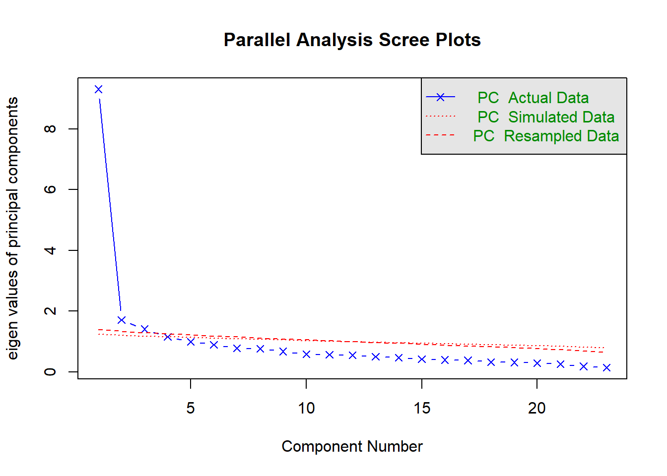
## Parallel analysis suggests that the number of factors = NA and the number of components = 3The Scree plot shows that the first factor accounts for a substantial amount of variance compared to the second and subsequent factors. There is a large drop from the first factor to the second (forming a clear “mountain side”), and mostly “rubble” afterwards, beginning with the second factor. This indicates that most co-variation in the items is explained by just one factor. However, Parallel Analysis reveals that there are 3 factors, as factors 2 and 3 explain significantly more variance than would be expected in random data of this size. From the Scree plot it is clear that factors 2 and 3 explain little variance (even if significant). Residuals will reveal which correlations are not well explained by just 1 factor, and might give us a clue why the 2nd and 3rd factors are required.
Step 4. Fitting and interpreting a single-factor model
Now let’s fit a single-factor model to the 23 Neuroticism items. We will again request the tetrachoric correlations (cor="tet") and the maximum likelihood estimation method (fm="ml").
## Factor Analysis using method =  ml
## Call: fa(r = EPQ[4:26], nfactors = 1, fm = "ml", cor = "tet")
## Standardized loadings (pattern matrix) based upon correlation matrix
##       ML1   h2   u2 com
## N_3  0.69 0.47 0.53   1
## N_7  0.65 0.43 0.57   1
## N_12 0.65 0.43 0.57   1
## N_15 0.52 0.27 0.73   1
## N_19 0.74 0.55 0.45   1
## N_23 0.66 0.44 0.56   1
## N_27 0.67 0.45 0.55   1
## N_31 0.69 0.48 0.52   1
## N_34 0.80 0.64 0.36   1
## N_38 0.65 0.42 0.58   1
## N_41 0.65 0.42 0.58   1
## N_47 0.40 0.16 0.84   1
## N_54 0.43 0.18 0.82   1
## N_58 0.58 0.34 0.66   1
## N_62 0.56 0.31 0.69   1
## N_66 0.50 0.25 0.75   1
## N_68 0.48 0.23 0.77   1
## N_72 0.69 0.48 0.52   1
## N_75 0.72 0.51 0.49   1
## N_77 0.67 0.45 0.55   1
## N_80 0.65 0.43 0.57   1
## N_84 0.43 0.18 0.82   1
## N_88 0.43 0.19 0.81   1
##
##                 ML1
## SS loadings    8.72
## Proportion Var 0.38
##
## Mean item complexity =  1
## Test of the hypothesis that 1 factor is sufficient.
##
## df null model =  253  with the objective function =  12.39 with Chi Square =  16995.3
## df of  the model are 230  and the objective function was  3.74
##
## The root mean square of the residuals (RMSR) is  0.08
## The df corrected root mean square of the residuals is  0.08
##
## The harmonic n.obs is  1374 with the empirical chi square  4262.77  with prob <  0
## The total n.obs was  1381  with Likelihood Chi Square =  5122.04  with prob <  0
##
## Tucker Lewis Index of factoring reliability =  0.678
## RMSEA index =  0.124  and the 90 % confidence intervals are  0.121 0.127
## BIC =  3459.01
## Fit based upon off diagonal values = 0.96
## Measures of factor score adequacy
##                                                    ML1
## Correlation of (regression) scores with factors   0.97
## Multiple R square of scores with factors          0.94
## Minimum correlation of possible factor scores     0.88
Run this command and examine the output. Try to answer the following questions (refer to instructional materials of your choice for help, I recommend McDonald’s “Test theory”). I will indicate which parts of the output you need to answer each question.
QUESTION 3. Examine the Standardized factor loadings. How do you interpret them? What is the “marker item” for the Neuroticism scale? [In the “Standardized loadings” output, the loadings are printed in “ML1” column. “ML” stands for the estimation method, “Maximum Likelihood”, and “1” stands for the factor number. Here we have only 1 factor, so only one column.]
QUESTION 4. Examine communalities and uniquenesses (look at h2 and u2 values in the table of “Standardized loadings”, respectively). What is communality and uniqueness and how do you interpret them?
QUESTION 5. What is the proportion of variance explained by the factor in all 23 items (total variance explained)? To answer this question, look for “Proportion Var” entry in the output (in a small table beginning with “SS loadings”).
Step 5. Assessing the model’s goodness of fit
Now let us examine the model’s goodness of fit (GOF). This output starts with the line “Test of the hypothesis that 1 factor is sufficient”. This is the hypothesis that the data complies with a single-factor model (“the model”). We are hoping to retain this hypothesis, therefore hoping for a larger p-value, definitely larger than 0.05, and ideally much larger. The output will also tell us about the “null model”, which is the model where all items are uncorrelated. We are obviously hoping to reject this null model, and obtain a very small p-value. Both of these models will be tested with the chi-square test, with their respective degrees of freedom. For our single-factor model, there are 230 degrees of freedom, because the model estimates 46 parameters (23 factor loadings and 23 uniquenesses), and there are 23*24/2=276 variances and covariances (sample moments) to estimate them. The degrees of freedom are therefore 276-46=230.
QUESTION 6. Is the chi-square for the tested model significant? Do you accept or reject the single-factor model? [Look for “Likelihood Chi Square” in the output.]
For now, I will ignore some other “fit indices” printed in the output. I will return to them in Exercises dealing with structural equation models (beginning with Exercise 16) .
Now let’s examine the model’s residuals. Residuals are the differences between the observed item correlations (which we computed earlier) and the correlations “reproduced” by the model – that is, correlations of item scores predicted by the model. In the model output printed on Console, we have the Root Mean Square Residual (RMSR), which is a summary measure of the size of residuals, and in a way it is like GOF “effect size” - independent of sample size. You can see that the RMSR=0.08, which is an acceptable value, indicating that the average residual is sufficiently small.
To obtain more detailed output of the residuals, we need to get access to all of the results produced by the function fa(). Call the function again, but this time, assign its results to a new object fit, which we can “interrogate” later.
Package psych has a nice function that pulls the residuals from the saved factor analysis results (object fit) and prints them in a user-friendly way. To remove item uniquenesses from the diagonal out of sight, use option diag=FALSE.
##      N_3   N_7   N_12  N_15  N_19  N_23  N_27  N_31  N_34  N_38  N_41
## N_3     NA
## N_7   0.09    NA
## N_12 -0.01  0.06    NA
## N_15  0.19  0.01 -0.11    NA
## N_19  0.00 -0.03  0.05 -0.09    NA
## N_23  0.09  0.03 -0.01  0.12 -0.07    NA
## N_27 -0.02 -0.01  0.11  0.03 -0.01  0.00    NA
## N_31 -0.07 -0.13 -0.10 -0.01 -0.01 -0.08 -0.05    NA
## N_34 -0.09 -0.02  0.04 -0.08  0.01 -0.04  0.01  0.16    NA
## N_38 -0.05 -0.06  0.05  0.01 -0.04 -0.01  0.06  0.01  0.09    NA
## N_41 -0.05 -0.08 -0.11  0.13 -0.03 -0.01 -0.06  0.19  0.06  0.01    NA
## N_47 -0.01 -0.06  0.07 -0.05 -0.05  0.05  0.04  0.02 -0.01  0.18 -0.03
## N_54  0.04  0.03 -0.06  0.11 -0.06 -0.02 -0.04  0.02 -0.03 -0.02  0.07
## N_58  0.14  0.14  0.00  0.03 -0.05  0.16 -0.01 -0.09 -0.11 -0.06 -0.10
## N_62  0.09  0.02 -0.07  0.09 -0.07  0.11 -0.04 -0.05 -0.05 -0.04  0.03
## N_66 -0.03 -0.07  0.13 -0.05  0.02  0.04  0.01 -0.07 -0.02  0.06 -0.10
## N_68  0.03  0.13 -0.04  0.05 -0.02  0.00  0.02 -0.11 -0.06 -0.02 -0.07
## N_72 -0.09  0.03  0.08 -0.13  0.10 -0.08  0.06  0.00  0.05 -0.01 -0.02
## N_75 -0.06 -0.02 -0.06  0.04 -0.04 -0.05 -0.09  0.26  0.04 -0.02  0.14
## N_77  0.07  0.02 -0.10  0.02 -0.04  0.11  0.02 -0.05 -0.08 -0.05 -0.03
## N_80 -0.08 -0.07  0.03 -0.18  0.29 -0.13  0.00  0.01  0.00 -0.04  0.00
## N_84  0.13  0.11  0.01 -0.06 -0.08  0.04  0.01 -0.11 -0.07 -0.04 -0.09
## N_88  0.08  0.07 -0.03  0.07  0.07  0.06 -0.02 -0.19 -0.01  0.03 -0.02
##      N_47  N_54  N_58  N_62  N_66  N_68  N_72  N_75  N_77  N_80  N_84
## N_47    NA
## N_54 -0.02    NA
## N_58  0.03  0.10    NA
## N_62 -0.10  0.03  0.04    NA
## N_66  0.13 -0.04 -0.04 -0.02    NA
## N_68 -0.12  0.07  0.06  0.12 -0.01    NA
## N_72  0.00 -0.16 -0.08 -0.06  0.07  0.01    NA
## N_75  0.03  0.09 -0.01 -0.02 -0.06 -0.09 -0.02    NA
## N_77 -0.09  0.08  0.05  0.26  0.04  0.10 -0.04 -0.04    NA
## N_80 -0.09 -0.06 -0.09 -0.13  0.05  0.01  0.14  0.02 -0.02    NA
## N_84  0.04  0.06  0.24  0.05 -0.02  0.09 -0.06 -0.08  0.04 -0.05    NA
## N_88  0.02 -0.04  0.07 -0.08  0.02 -0.01 -0.08 -0.04 -0.03  0.05  0.13
## [1]    NA
For a large residuals matrix as we have here, it is convenient to summarize the results with a histogram:
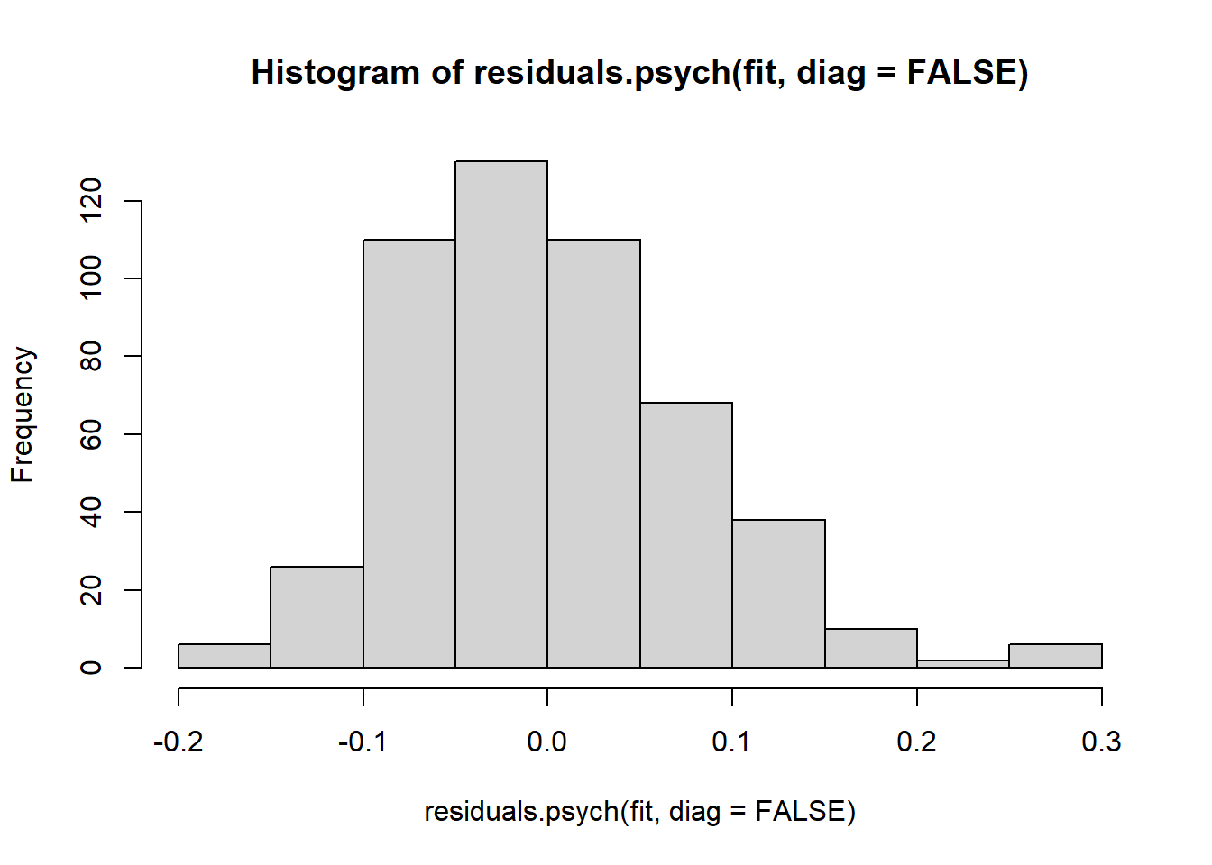
QUESTION 7. Examine the residuals. What can you say about them? Are there any large residuals? (Hint. Interpret the size of residuals as you would the size of correlation coefficients.)
Step 6. Estimating scale reliability using McDonald’s omega
Since we have confirmed relative homogeneity of the Neuroticism scale, we can legitimately estimate its reliability using coefficients alpha or omega. In Exercise 6, we already computed alpha from tetrachoric correlations for this scale, so you can refer to that instruction for detail. I will simply quote the result we obtained there, alpha=0.93.
To obtain omega, call function omega(), specifying the number of factors (nfactors=1). You need this because various versions of coefficient omega exist for multi-factor models, but you only need the estimate for a homogeneous test, “Omega Total”.
## Loading required namespace: GPArotation## Omega_h for 1 factor is not meaningful, just omega_t## Warning in schmid(m, nfactors, fm, digits, rotate = rotate, n.obs = n.obs, :
## Omega_h and Omega_asymptotic are not meaningful with one factor## Omega
## Call: omegah(m = m, nfactors = nfactors, fm = fm, key = key, flip = flip,
## digits = digits, title = title, sl = sl, labels = labels,
## plot = plot, n.obs = n.obs, rotate = rotate, Phi = Phi, option = option,
## covar = covar)
## Alpha: 0.93
## G.6: 0.95
## Omega Hierarchical: 0.93
## Omega H asymptotic: 1
## Omega Total 0.93
##
## Schmid Leiman Factor loadings greater than 0.2
## g F1* h2 h2 u2 p2 com
## N_3 0.70 0.50 0.50 0.50 1 1
## N_7 0.66 0.44 0.44 0.56 1 1
## N_12 0.65 0.42 0.42 0.58 1 1
## N_15 0.53 0.28 0.28 0.72 1 1
## N_19 0.74 0.54 0.54 0.46 1 1
## N_23 0.68 0.46 0.46 0.54 1 1
## N_27 0.67 0.45 0.45 0.55 1 1
## N_31 0.67 0.45 0.45 0.55 1 1
## N_34 0.79 0.62 0.62 0.38 1 1
## N_38 0.65 0.42 0.42 0.58 1 1
## N_41 0.64 0.41 0.41 0.59 1 1
## N_47 0.40 0.16 0.84 1 1
## N_54 0.44 0.19 0.81 1 1
## N_58 0.60 0.36 0.36 0.64 1 1
## N_62 0.56 0.32 0.32 0.68 1 1
## N_66 0.50 0.25 0.25 0.75 1 1
## N_68 0.49 0.24 0.24 0.76 1 1
## N_72 0.68 0.46 0.46 0.54 1 1
## N_75 0.71 0.50 0.50 0.50 1 1
## N_77 0.68 0.47 0.47 0.53 1 1
## N_80 0.64 0.41 0.41 0.59 1 1
## N_84 0.44 0.19 0.81 1 1
## N_88 0.44 0.19 0.81 1 1
##
## With Sums of squares of:
## g F1* h2
## 8.7 0.0 3.7
##
## general/max 2.38 max/min = 1.32278e+16
## mean percent general = 1 with sd = 0 and cv of 0
## Explained Common Variance of the general factor = 1
##
## The degrees of freedom are 230 and the fit is 3.74
##
## The root mean square of the residuals is 0.08
## The df corrected root mean square of the residuals is 0.08
##
## Compare this with the adequacy of just a general factor and no group factors
## The degrees of freedom for just the general factor are 230 and the fit is 3.74
##
## The root mean square of the residuals is 0.08
## The df corrected root mean square of the residuals is 0.08
##
## Measures of factor score adequacy
## g F1*
## Correlation of scores with factors 0.97 0
## Multiple R square of scores with factors 0.94 0
## Minimum correlation of factor score estimates 0.88 -1
##
## Total, General and Subset omega for each subset
## g F1*
## Omega total for total scores and subscales 0.93 0.93
## Omega general for total scores and subscales 0.93 0.93
## Omega group for total scores and subscales 0.00 0.00QUESTION 8. What is the “Omega Total” for Conduct Problems scale score? How does it compare with the alpha for this scale?
Step 7. Saving your work
After you finished work with this exercise, save your R script by pressing the Save icon in the script window. Give the script a meaningful name, for example “EPQ_N scale homogeneity analyses”. When closing the project by pressing File / Close project, make sure you select Save when prompted to save your ‘Workspace image’ (with extension .RData).
8.3 Solutions
Q1. Both sets of correlations support the suitability for factor analysis because they are all positive and relatively similar in size, as expected for items measuring the same thing. The tetrachoric correlations are larger than the product-moment correlations. This is not surprising given that the product-moment correlations tend to underestimate the strength of the relationships between binary items.
Q2. MSA = 0.92. The data are “marvelous” for factor analysis according to the Kaiser’s guidelines.
Q3. Standardized factor loadings reflect the number of Standard Deviations by which the item score will change per 1 SD change in the factor score. The higher the loading, the more sensitive the item is to the change in the factor. Standardised factor loadings in the single-factor model are also correlations between the factor and the items (just like beta coefficients in the simple regression). For the Neuroticism scale, factor loadings range between 0.40 and 0.80. Factor loadings over 0.5 can be considered reasonably high. The marker item is N_34 with the loading 0.80 (highest loading). This item, “Are you a worrier”, is central to the meaning of the common factor (and supports the hypothesis that the construct measured by this item set is indeed Neuroticism).
Q4. Communality is the variance in the item due to the common factor, and uniqueness is the unique item variance. In standardised factor solutions (which is what function fa() prints), communality is the proportion of variance in the item due to the factor, and uniqueness is the remaining proportion (1-communality). Looking at the printed values, between 16% and 64% of variance in the items is due to the common factor.
Q5. The factor accounts for 38% of the variability in the 23 Neuroticism items.
Q6. The chi-square test is highly significant, which means the null hypothesis (that the single-factor model holds in the population) must be rejected. However, the chi-square test is sensitive to the sample size, and even very good models are rejected when large samples (like the one tested here, N=1381) are used to test them.
Q7. The vast majority of residuals are between -0.1 and 0.1. However, there are few large residuals, above 0.2. For instance, the largest residual correlation (0.29) is between N_19 (“Are your feelings easily hurt?”) and N_80 (“Are you easily hurt when people find fault with you or the work you do?). This is a clear case of so-called local dependence - when the dependency between two items remains even after accounting for the common factor. It is not surprising to find local dependence in two items with such a similar wording. These items have far more in common than they have with other items. Beyond the common factor that they share with other items, these item also share some of their unique parts. Another large residual, 0.26, is between N_31 (”Would you call yourself a nervous person?“) and N_75 (”Do you suffer from “nerves”?“). Again, there is a clear similarity of wording in these two items. These cases of local dependence might be responsible for the 2nd and 3rd factors we found in Parallel Analysis.
Q8. Omega Total = 0.93, and is the same as Alpha = 0.93 (at least to the second decimal place). Coefficient alpha can only be lower than omega, and they are equal when all factor loadings are equal. Here, not all loadings are equal, but most are very similar, resulting in very similar alpha and omega.