Exercise 21 Growth curve modelling of longitudinal measurements
| Data file | ALSPAC.csv |
| R package | lavaan, lcsm, psych |
21.1 Objectives
In this exercise, you will perform growth curve modelling of longitudinal measurements of child development. These will be measurements of weight or height. Redeeming features of such measures are that they have little or no error of measurement (unlike most psychological data), and that they are continuous variables at the highest level of measurement - ratio scales. These features enable analysis of growth patterns without being concerned about the measurement, and thus focus on the structural part of the model. You will practice plotting growth trajectories and modelling these trajectories with growth curve models with random intercept and random slopes (both linear and quadratic).
21.2 Study of child growth in a longitudinal repeated-measures design spanning 8 years
First, I must make some acknowledgements. Data and many ideas for the analyses in this exercise are due to Dr Jon Heron of Bristol Medical School. This data example was first presented in a summer school that Dr Heron and other dear colleagues of mine taught at the University of Cambridge in 2011.
Data for this exercise comes from the Avon Longitudinal Study of Parents and Children (ALSPAC), also known as “Children of the Nineties”. This is a population-based prospective birth-cohort study of ~14,000 children and their parents, based in South-West England. For a child to be eligible for inclusion in the study, their mother had to be resident in Avon and have an expected date of delivery between April 1st 1991 and December 31st 1992.
We will analyse some basic growth measurements taken in clinics attended at approximate ages 7, 9, 11, 13 and 15 years. There are N=802 children in the data file ALSPAC.csv that we will consider here, 376 boys and 426 girls.
The analysis dataset is in wide-data format so that each repeated measure is a different variable (e.g. ht7, ht9, ht11, …). The file contains the following variables:
| ht 7/9/11/13/15 | Child height (cm) at the 7, 9, 11, 13 and 15 year clinics |
| wt 7/9/11/13/15 | Child weight (kg) at each clinic |
| bmi 7/9/11/13/15 | Child body mass index at each clinic |
| age 7/9/11/13/15 | Child actual age at measurement (months) at each clinic |
| female | Sex dummy (coded 1 for girl, and 0 for boy) |
| bwt | Birth weight (kg) |
21.3 Worked Example - Fitting growth curve models to longitudinal measurements of child’s weight
To complete this exercise, you need to repeat the analysis of weight measurements from a worked example below, and answer some questions. Once you are confident, you may want to explore the height measurements independently.
Step 1. Reading and examining data
Download file ALSPAC.csv, save it in a new folder (e.g. “Growth curve model of ALSPAC data”), and create a new project in this new folder.
Import the data (which is in the comma-separated-values format) into a new data frame. I will call it ALSPAC.
First, produce and examine the descriptive statistics to learn about the coverage and spread of measurements. As you can see, there are no missing data.
##        vars   n    mean      sd  median trimmed     mad    min     max   range
## id        1 802 1913.68 1120.48 1929.00 1907.45 1447.02   3.00 3883.00 3880.00
## ht7       2 802  125.62    5.26  125.50  125.55    5.26 111.40  140.80   29.40
## wt7       3 802   25.58    4.09   25.00   25.23    3.56  16.60   43.40   26.80
## bmi7      4 802   16.14    1.88   15.79   15.94    1.50  10.85   27.78   16.94
## age7      5 802   89.56    2.05   89.00   89.27    1.48  86.00  109.00   23.00
## ht9       6 802  139.26    6.14  139.00  139.18    6.08 120.90  163.00   42.10
## wt9       7 802   34.13    6.70   32.90   33.54    6.08  21.40   61.80   40.40
## bmi9      8 802   17.50    2.62   16.89   17.22    2.29  13.02   29.84   16.82
## age9      9 802  117.71    3.22  117.00  117.28    2.97 113.00  136.00   23.00
## ht11     10 802  150.55    6.99  150.40  150.41    7.41 131.10  174.20   43.10
## wt11     11 802   43.11    9.23   41.20   42.34    8.60  24.00   76.20   52.20
## bmi11    12 802   18.89    3.15   18.14   18.58    2.88  12.44   31.69   19.25
## age11    13 802  140.54    2.24  140.00  140.39    1.48 133.00  154.00   21.00
## ht13     14 802  157.05    7.28  156.80  156.99    7.26 136.00  180.30   44.30
## wt13     15 802   48.77    9.98   47.50   48.08    9.56  25.70   87.30   61.60
## bmi13    16 802   19.68    3.26   19.04   19.38    2.91  13.07   32.02   18.95
## age13    17 802  153.29    2.35  153.00  153.23    1.48 138.00  169.00   31.00
## ht15     18 802  169.09    8.15  168.50  168.88    8.15 147.40  192.20   44.80
## wt15     19 802   60.87   11.17   58.80   59.83    8.90  35.20  119.10   83.90
## bmi15    20 802   21.25    3.36   20.62   20.86    2.73  14.09   38.23   24.14
## age15    21 802  185.05    3.33  184.00  184.55    1.48 177.00  203.00   26.00
## female   22 802    0.53    0.50    1.00    0.54    0.00   0.00    1.00    1.00
## bwt      23 802    3.42    0.54    3.45    3.44    0.46   0.82    5.14    4.31
##         skew kurtosis    se
## id      0.01    -1.22 39.57
## ht7     0.11    -0.23  0.19
## wt7     0.99     1.60  0.14
## bmi7    1.34     3.18  0.07
## age7    4.47    29.62  0.07
## ht9     0.14    -0.12  0.22
## wt9     0.89     0.81  0.24
## bmi9    1.05     1.17  0.09
## age9    1.63     4.07  0.11
## ht11    0.16    -0.23  0.25
## wt11    0.80     0.42  0.33
## bmi11   0.96     0.85  0.11
## age11   0.88     2.49  0.08
## ht13    0.06    -0.15  0.26
## wt13    0.67     0.31  0.35
## bmi13   0.90     0.69  0.12
## age13   0.39     5.43  0.08
## ht15    0.26    -0.24  0.29
## wt15    1.13     2.28  0.39
## bmi15   1.35     2.81  0.12
## age15   2.27     7.49  0.12
## female -0.12    -1.99  0.02
## bwt    -0.56     2.10  0.02
You may also want to examine data by sex, because there might be differences in growth patters between boys and girls. Do this independently using function describeBy(ALSPAC, group="female") from package psych.
Step 2. Plotting individual development trajectories
We begin with visualizing the data. Perhaps the most useful way of looking at individuals’ development over time is to connect individual values for each time point, thus building “trajectories” of change . Package lcsm offers a nice function plot_trajectories() that does exactly that:
## load the lcsm package
library(lcsm)

## plotting individual WEIGHT trajectories
plot_trajectories(data = ALSPAC,
                  id_var = "id",
                  var_list = c("wt7", "wt9", "wt11", "wt13", "wt15"),
                  xlab = "Age in years",
                  ylab = "Weight in kilograms",
                  line_colour = "black")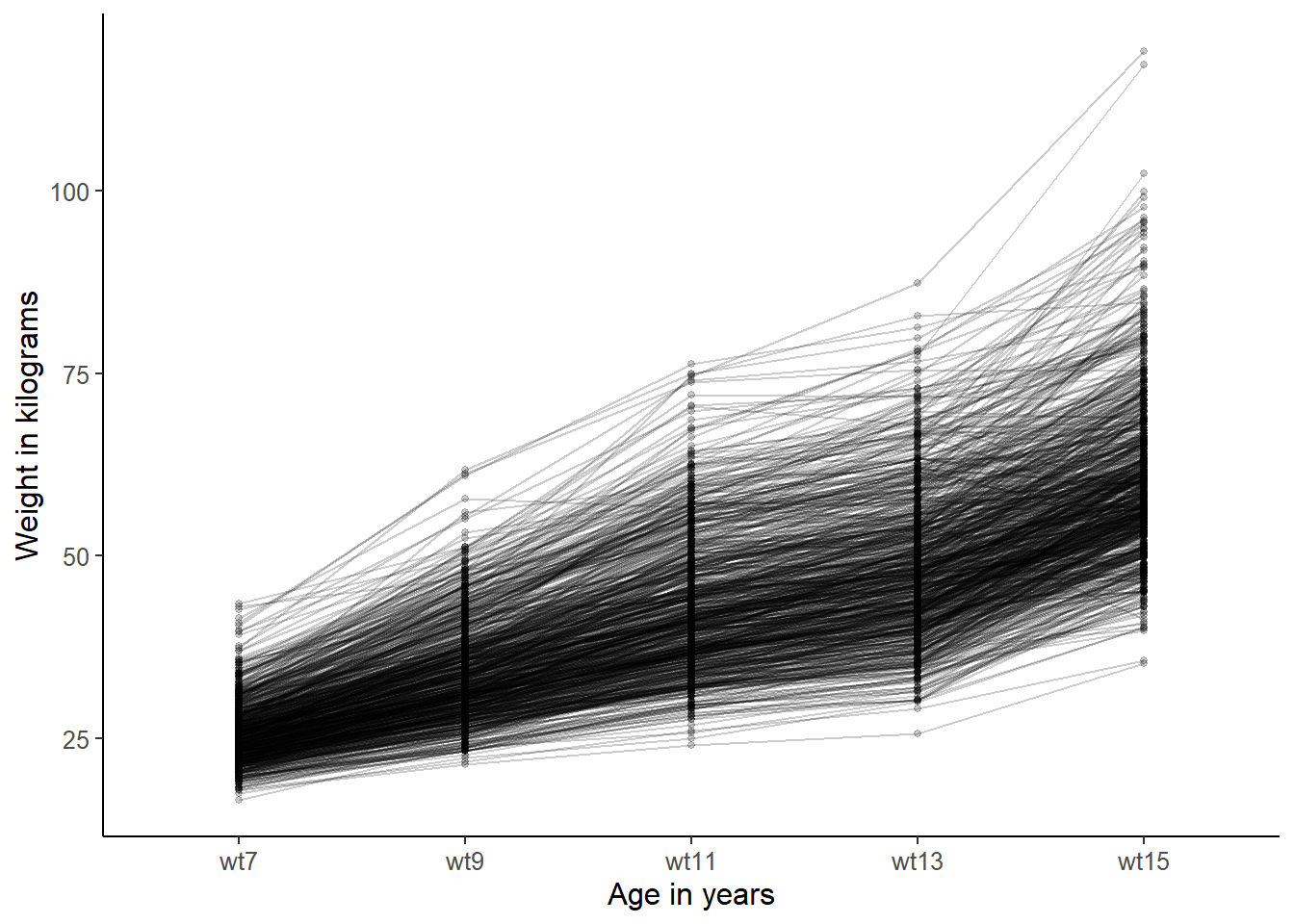
Each line on the graph represents a child, and you can see how weight of each child changes over time. You can see that there is strong tendency to weight increase, as you may expect, but also quite a lot of variation in the starting weight and also in the rate of change. You can perhaps see an overall tendency for almost linear growth between ages 7 and 11, but then slowing as children reach 13,and then a fast acceleration between 13 and 15 (puberty).
You may, however, suspect that there might be systematic differences between trajectories of boys and girls. To address this, we can plot the sexes separately.
## trajectories for boys only
plot_trajectories(data = ALSPAC[ALSPAC$female==0, ],
                  id_var = "id",
                  var_list = c("wt7", "wt9", "wt11", "wt13", "wt15"),
                  xlab = "Age in years",
                  ylab = "Weight in kilograms",
                  line_colour = "blue")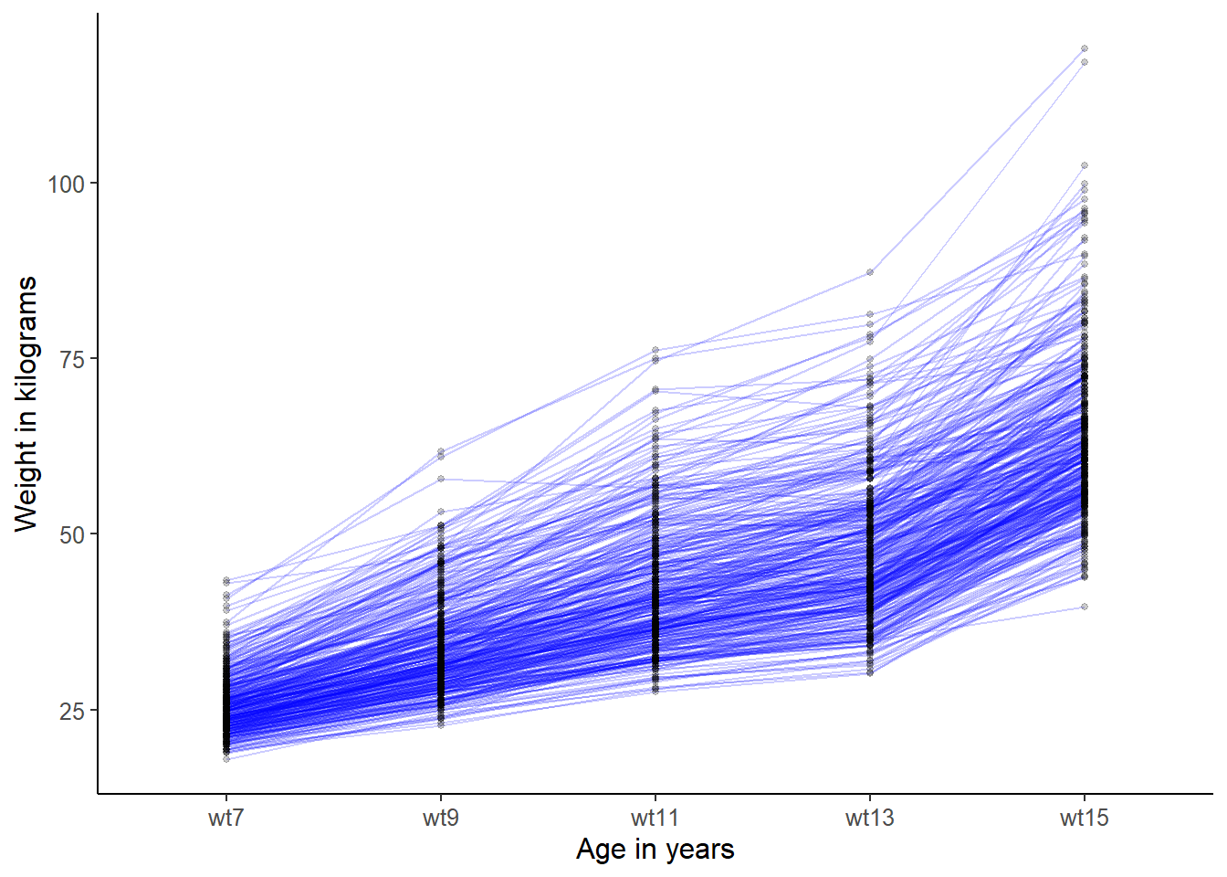
QUESTION 1. Using the syntax above as guide, plot the individual trajectories for girls, in a different colour (say, “red”). Are the trajectories for girls look similar to trajectories for boys?
Step 3. Specifying and fitting a linear growth model to 4 repeated measurements
Now we are ready to start growth curve (GC) modelling. I will demonstrate how to fit GC models to the repeated measures of weight for the boys only (and you can try to fit these for girls independently).
First we note that each trajectory (individual child) can be characterized by its own baseline and rate of increase. For instance, some boys start at below average weight and stay low. Some start average but gain weight quickly. Some start high and gain weight at an average rate. And all combinations of the baseline and growth rate are of course possible.
When the developmental process is of interest, longitudinal observations can be described in terms of trajectories of change. For every child, instead of all the repeated observations, we may consider:
- The intercept (expected weight at baseline)
- The slope (linear rate of increase in weight per year)
One aim of such models is to summarize growth through new variables, which can be used in analyses as predictors, or outcomes, or mediators, etc. Another aim is to test if a linear model is sufficient to describe the growth process. In linear models, any deviations from linear trajectories are considered as random errors. In the ALSPAC example, the linear trend is visible between ages 7 and 11, but the rate of change seems to slow down as children reach age 13 (we will test it formally when looking at the model fit).
So, we will attempt to describe the observed change occurring between ages 7 and 13 (for simplicity, I will not include age 15 as different growth factors come to play then). We will describe the data through two new random variables - intercept and slope, representing each child’s trajectory through his unique baseline and rate of change. We can assume that these variables are normally distributed, so there are average, low and high baselines, and average, low and high rates of change. Most children are expected to be in the average range, and a few will have extremely high or low values. So the idea is to describe systematic variability in the data through a model with only 2 variables (which would necessarily be quite a substantial simplification from the original 4 variables).
If linear rate of change holds, then each observation could be described as follows:
wt7 = intercept + e7
wt9 = intercept + 2*slope + e9
wt11 = intercept + 4*slope + e11
wt13 = intercept + 6*slope + e13
The slope (latent variable) is the rate of change (kg per year), and coefficients in front of this variable represent the number of years passing from the first measurement at age 7. Obviously, at age 7 the coefficient for slope is 0. The intercept (latent variable) represents the predicted weight at 7 for each child (this may or may not correspond to the child’s actual weight at 7). Of course weights predicted by this rather crude model will not describe the data exactly, and that is why we need errors of prediction (variables e7 to e13).
The hypothesized linear growth curve model can be depicted as in figure below.
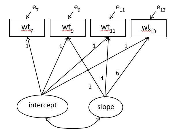
Figure 21.1: Linear growth curve model for 4 repeated bodyweight measurements
To code this model, we describe the growth variables - intercept i and slope s - using the lavaan syntax conventions. We use the shorthand symbol =~ for is measured by and use * for fixing the “loading” coefficients as the equations above specify.
Linear <- '  # linear growth model with 4 measurements
# intercept and slope with fixed coefficients
i =~ 1*wt7 + 1*wt9 + 1*wt11 + 1*wt13
s =~ 0*wt7 + 2*wt9 + 4*wt11 + 6*wt13
'
To fit this GC model, lavaan has function growth(). We need to pass to it: the model (model=Linear, or simply Linear if you put this argument first), and the data.
# do not forget to load the lavaan package!
library(lavaan)

# fit the growth model for boys only
fitL <- growth(Linear, data=ALSPAC[ALSPAC$female==0, ])

# include additional fit indices
summary(fitL, fit.measures=TRUE)
## lavaan 0.6-19 ended normally after 94 iterations
##
## Estimator ML
## Optimization method NLMINB
## Number of model parameters 9
##
## Number of observations 376
##
## Model Test User Model:
##
## Test statistic 272.201
## Degrees of freedom 5
## P-value (Chi-square) 0.000
##
## Model Test Baseline Model:
##
## Test statistic 2260.736
## Degrees of freedom 6
## P-value 0.000
##
## User Model versus Baseline Model:
##
## Comparative Fit Index (CFI) 0.881
## Tucker-Lewis Index (TLI) 0.858
##
## Loglikelihood and Information Criteria:
##
## Loglikelihood user model (H0) -4111.927
## Loglikelihood unrestricted model (H1) -3975.826
##
## Akaike (AIC) 8241.854
## Bayesian (BIC) 8277.220
## Sample-size adjusted Bayesian (SABIC) 8248.665
##
## Root Mean Square Error of Approximation:
##
## RMSEA 0.377
## 90 Percent confidence interval - lower 0.340
## 90 Percent confidence interval - upper 0.416
## P-value H_0: RMSEA <= 0.050 0.000
## P-value H_0: RMSEA >= 0.080 1.000
##
## Standardized Root Mean Square Residual:
##
## SRMR 0.096
##
## Parameter Estimates:
##
## Standard errors Standard
## Information Expected
## Information saturated (h1) model Structured
##
## Latent Variables:
## Estimate Std.Err z-value P(>|z|)
## i =~
## wt7 1.000
## wt9 1.000
## wt11 1.000
## wt13 1.000
## s =~
## wt7 0.000
## wt9 2.000
## wt11 4.000
## wt13 6.000
##
## Covariances:
## Estimate Std.Err z-value P(>|z|)
## i ~~
## s 3.714 0.354 10.502 0.000
##
## Intercepts:
## Estimate Std.Err z-value P(>|z|)
## i 25.882 0.222 116.465 0.000
## s 3.982 0.067 59.129 0.000
##
## Variances:
## Estimate Std.Err z-value P(>|z|)
## .wt7 0.861 0.403 2.138 0.033
## .wt9 3.836 0.383 10.014 0.000
## .wt11 5.488 0.664 8.262 0.000
## .wt13 12.342 1.492 8.270 0.000
## i 17.767 1.398 12.706 0.000
## s 1.508 0.127 11.883 0.000Examine the output and answer the following questions.
QUESTION 2. How many parameters are there to estimate? What are they? How many known pieces of information (sample moments) are there in the data? What are the degrees of freedom and how are they calculated?
QUESTION 3. Interpret the chi-square statistic. Do you retain or reject the model?
QUESTION 4. Interpret the RMSEA, CFI and SRMR. What do you conclude about the model fit?
Next, let’s investigate the reason for model misfit. Ask for model residuals (which are differences between the observed and the expected (model-implied) summary statistics, such as means, variances and covariances). To evaluate the effect size of the residuals, ask for type="cor", which will be based on standardized variables (and the covariances will turn into correlations).
## $type
## [1] "cor.bollen"
##
## $cov
##         wt7    wt9   wt11   wt13
## wt7   0.000
## wt9   0.011  0.000
## wt11 -0.007  0.016  0.000
## wt13  0.008 -0.001  0.036  0.000
##
## $mean
##    wt7    wt9   wt11   wt13
## -0.020  0.043  0.089 -0.151
Under $cov, we have the differences between actual minus expected covariances of the repeated measures. This information can help find weaknesses in the model by finding residuals that are large compared to the rest. No large residuals (greater than 0.1) can be seen in the output.
Under $mean, we have the differences between actual minus estimated means. The residuals are largest for the last measurement point (wt13), suggesting that a linear model might not be adequately capturing the longitudinal trend in weight. The negative sign of the residual means that the model predicts larger weight at age 13 than actually observed. We conclude that the linear model fails to describe adequately the slowing down of growth towards the age 13.
Step 4. Specifying and fitting a quadratic growth model to 4 repeated measurements
To address the inadequate fit of the linear model, we will add a quadratic slope, which will capture the non-linear trend (slowing down of growth) that we observed on the trajectory plots and also by examining residuals.
Now we will describe each observation as a weighted sum of the intercept, the slope and the quadratic slope:
wt7 = intercept + e7
wt9 = intercept + 2*slope + 4*qslope + e9
wt11 = intercept + 4*slope + 16*qslope + e11
wt13 = intercept + 6*slope + 36*qslope + e13
The qslope (latent variable) is the quadratic rate of change (squared kg per year), and coefficients in front of this variable represent the squared number of years passing from the first measurement at age 7. Obviously, at age 7 the coefficient for quadratic slope is 0.
Quadratic <- '  # quadratic growth model for 4 measurements
# intercept and slope with fixed coefficients
i =~ 1*wt7 + 1*wt9 + 1*wt11 + 1*wt13
s =~ 0*wt7 + 2*wt9 + 4*wt11 + 6*wt13
q =~ 0*wt7 + 4*wt9 + 16*wt11 + 36*wt13
'
# fit the growth model, boys only
fitQ <- growth(Quadratic, data=ALSPAC[ALSPAC$female==0, ])
## Warning: lavaan->lav_object_post_check():
## some estimated ov variances are negative## Warning: lavaan->lav_object_post_check():
## covariance matrix of latent variables is not positive definite ; use
## lavInspect(fit, "cov.lv") to investigate.It seems we have a problem. The program is telling us that ’covariance matrix of latent variables is not positive definite”. Let’s examine the summary output:
## lavaan 0.6-19 ended normally after 118 iterations
##
##   Estimator                                         ML
##   Optimization method                           NLMINB
##   Number of model parameters                        13
##
##   Number of observations                           376
##
## Model Test User Model:
##
##   Test statistic                                52.148
##   Degrees of freedom                                 1
##   P-value (Chi-square)                           0.000
##
## Parameter Estimates:
##
##   Standard errors                             Standard
##   Information                                 Expected
##   Information saturated (h1) model          Structured
##
## Latent Variables:
##                    Estimate  Std.Err  z-value  P(>|z|)
##   i =~
##     wt7               1.000
##     wt9               1.000
##     wt11              1.000
##     wt13              1.000
##   s =~
##     wt7               0.000
##     wt9               2.000
##     wt11              4.000
##     wt13              6.000
##   q =~
##     wt7               0.000
##     wt9               4.000
##     wt11             16.000
##     wt13             36.000
##
## Covariances:
##                    Estimate  Std.Err  z-value  P(>|z|)
##   i ~~
##     s                 7.704    1.281    6.015    0.000
##     q                -0.657    0.144   -4.548    0.000
##   s ~~
##     q                -0.380    0.053   -7.159    0.000
##
## Intercepts:
##                    Estimate  Std.Err  z-value  P(>|z|)
##     i                25.593    0.218  117.646    0.000
##     s                 4.566    0.111   41.264    0.000
##     q                -0.153    0.014  -10.670    0.000
##
## Variances:
##                    Estimate  Std.Err  z-value  P(>|z|)
##    .wt7               4.747    1.867    2.543    0.011
##    .wt9              -0.167    0.983   -0.170    0.865
##    .wt11              9.494    1.432    6.629    0.000
##    .wt13            -17.604    4.541   -3.877    0.000
##     i                13.365    2.077    6.435    0.000
##     s                 2.965    0.518    5.726    0.000
##     q                 0.093    0.012    7.641    0.000
It shows that two residual variances, .wt9 and .wt13, are negative. This is obviously a problem, and could be a sign of model “overfitting”, when there are too many parameters estimated in the model. Indeed, this model estimates 13 parameters on 14 sample moments and has only 1 degree of freedom.
Examining the output again, we can see that the variance of q (quadratic slope) is only 0.093, which is very small compared to the variances of other growth factors i and s. A good way to reduce the number of parameters then is to fix the variance of q to 0, making it a fixed rather than a random effect. The quadratic slope will have the same effect on everyone’s trajectory (it will have the mean but no variance). And if q has no variance, it obviously should have zero covariance with the other growth factors i and s, so we fix those covariances to 0 as well. Here is the modified model:
QuadraticFixed <- paste(Quadratic, '
# the quadratic effect is fixed rather than random
q ~~ 0*q
q ~~ 0*i
q ~~ 0*s
')

fitQF <- growth(QuadraticFixed, data=ALSPAC[ALSPAC$female==0, ])

summary(fitQF, fit.measures=TRUE)
## lavaan 0.6-19 ended normally after 120 iterations
##
## Estimator ML
## Optimization method NLMINB
## Number of model parameters 10
##
## Number of observations 376
##
## Model Test User Model:
##
## Test statistic 154.874
## Degrees of freedom 4
## P-value (Chi-square) 0.000
##
## Model Test Baseline Model:
##
## Test statistic 2260.736
## Degrees of freedom 6
## P-value 0.000
##
## User Model versus Baseline Model:
##
## Comparative Fit Index (CFI) 0.933
## Tucker-Lewis Index (TLI) 0.900
##
## Loglikelihood and Information Criteria:
##
## Loglikelihood user model (H0) -4053.263
## Loglikelihood unrestricted model (H1) -3975.826
##
## Akaike (AIC) 8126.526
## Bayesian (BIC) 8165.822
## Sample-size adjusted Bayesian (SABIC) 8134.095
##
## Root Mean Square Error of Approximation:
##
## RMSEA 0.317
## 90 Percent confidence interval - lower 0.275
## 90 Percent confidence interval - upper 0.360
## P-value H_0: RMSEA <= 0.050 0.000
## P-value H_0: RMSEA >= 0.080 1.000
##
## Standardized Root Mean Square Residual:
##
## SRMR 0.072
##
## Parameter Estimates:
##
## Standard errors Standard
## Information Expected
## Information saturated (h1) model Structured
##
## Latent Variables:
## Estimate Std.Err z-value P(>|z|)
## i =~
## wt7 1.000
## wt9 1.000
## wt11 1.000
## wt13 1.000
## s =~
## wt7 0.000
## wt9 2.000
## wt11 4.000
## wt13 6.000
## q =~
## wt7 0.000
## wt9 4.000
## wt11 16.000
## wt13 36.000
##
## Covariances:
## Estimate Std.Err z-value P(>|z|)
## i ~~
## q 0.000
## s ~~
## q 0.000
## i ~~
## s 3.384 0.336 10.062 0.000
##
## Intercepts:
## Estimate Std.Err z-value P(>|z|)
## i 25.786 0.221 116.892 0.000
## s 4.701 0.092 51.035 0.000
## q -0.155 0.013 -12.161 0.000
##
## Variances:
## Estimate Std.Err z-value P(>|z|)
## q 0.000
## .wt7 0.317 0.395 0.802 0.422
## .wt9 4.626 0.418 11.068 0.000
## .wt11 5.460 0.612 8.919 0.000
## .wt13 5.874 1.109 5.296 0.000
## i 17.981 1.385 12.979 0.000
## s 1.465 0.118 12.457 0.000Now the model runs and produces admissible parameter values.
QUESTION 5. How many degrees of freedom does this model have? How does it compare to the random effect model Quadratic?
QUESTION 6. Interpret the chi-square statistic. How does it compare to the Linear model?
Step 5. Interpreting results of the growth curve model
Now we have a reasonably fitting model, at least according to the SRMR (0.072) and CFI (0.933), we can interpret the growth factors.
The section Intercepts presents the means of i, s and q, which we might refer to as the fixed-effect part of the model. We interpret these as follows:
The average 7-year-old boy in the population starts off with a body weight of 25.786kg, and that weight then increases by about 4.7kg per year, with an adjustment of -0.155 in the first year, and -0.155 times the number of years squared in each consecutive year. Therefore, the adjustment gets bigger as the time goes by, slowing the linear rate of growth.
The sections Variances and Covariances describe the random-effects part of the model, or the variances and covariance of our growth factors i and s. There is a strong positive covariance 3.384 indicating that larger children at age 7 tend to gain weight at a faster rate than smaller children. There is also considerable variation in both intercept (var(i)=17.981) and linear slope (var(s)=1.465) as evidenced by the plot of the raw data from earlier.
Finally, we can see the individual values on the growth factors (numbers describing intercept and slope for each boy’s individual trajectory). Package lavaan has function lavPredict(), which will compute these values for each boy in the sample. You need to apply this function to the result of fitting our best model with fixed quadratic effect, fitQF.
##             i        s          q
## [1,] 22.58784 3.984493 -0.1548515
## [2,] 21.08919 3.667423 -0.1548515
## [3,] 29.87843 5.794145 -0.1548515
## [4,] 27.29049 4.850545 -0.1548515
## [5,] 28.26804 5.018105 -0.1548515
## [6,] 23.54283 3.867593 -0.1548515
You can see that there are 3 values for each boy - i, s and q. While i and s vary between individuals, q is constant because we set it up as a fixed effect. You can plot histograms of the intercept and linear slope values as follows:
## plot the growth factors distributions
hist(lavPredict(fitQF)[,"i"], main="Random Intercept values",
                              xlab="Expected weight in kg at baseline")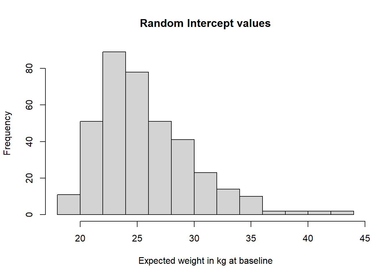
hist(lavPredict(fitQF)[,"s"], main="Random Linear slope values",
                              xlab="Expected rate of growth in kg per year")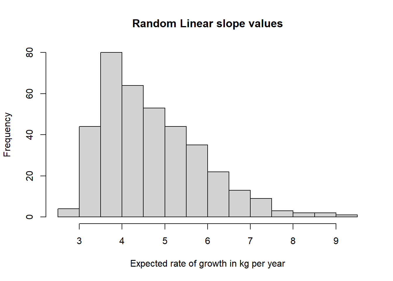
Both distributions have positive skews, with outliers located on the high end of the weight scale at baseline, and the high end of the weight gain per year.
Step 6. Investigating covariates of the growth factors
Finally, to give you an idea about how the random growth factors can be used in research, I will provide a simple illustration of a growth model with covariates. As we have the sex variable in the data set, we can easily investigate whether the child’s sex has any effect on body weight trajectories at this age (between 7 and 13). To this end, we simply regress our random growth factors, i and s on the sex dummy variable, female. We add the following line to the model QuadraticFixed:
QuadraticFixedSex <- paste(QuadraticFixed, '
# sex influences intercept and slope?
i ~ female
s ~ female
')

# Now we fit the model to ALL cases, boys and girls!
fitQFS <- growth(QuadraticFixedSex, data=ALSPAC)
Run the model and interpret the results.
QUESTION 7. Does child’s sex have a significant effect on the growth intercept? Who starts off with higher weight - boys or girls? Does sex have an effect on the linear slope? Who gains weight at a higher rate - boys or girls?
Step 7. Saving your work
After you finished work with this exercise, save your R script with a meaningful name, for example “Growth curve model of body weights”. To keep all of the created objects, which might be useful when revisiting this exercise, save your entire ‘work space’ when closing the project. Press File / Close project, and select “Save” when prompted to save your ‘Workspace image’.
21.4 Further practice - Testing growth curve models for girls
To practice further, fit a latent autoregressive path model to the girls’ body weights, and interpret the results.
21.5 Solutions
Q1.
# girls only
plot_trajectories(data = ALSPAC[ALSPAC$female==1, ],
id_var = "id",
var_list = c("wt7", "wt9", "wt11", "wt13", "wt15"),
xlab = "Age in years",
ylab = "Weight in kilograms",
line_colour = "red")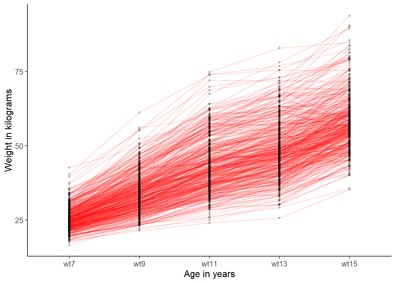 The trajectories for girls look quite similar to trajectories for boys. The spread is quite similar and the shapes are overall similar. Note that the scale of the y axis (weight) are different, so that the girls’ spread seems greater when in fact it is not.
Q2. The output prints that the “Number of model parameters” is 9, which are made up of 2 variances of latent variables i and S, 1 covariance of i and s, 2 intercepts of i and s, and 4 error (residual) variances of observed variables (.wt7, .wt9, wt11, and .wt13). There are 4 observed variables, therefore 4x(4+1)/2 = 10 sample moments in the variance/covariance matrix, plus 4 means, in total 14 sample moments. Then, the degrees of freedom is 5 (as lavaan tells you), calculated as 14(moments) – 9(parameters) = 5(df).
Q3. The chi-square test (Chi-square = 272.201, Degrees of freedom = 5) suggests rejecting the model because it is extremely unlikely (P-value < 0.001) that the observed data could emerge from the population in which the model is true.
Q4 The CFI = 0.881 falls short of acceptable levels of 0.9 or above; the RMSEA = 0.377 falls well short of acceptable levels of 0.08 and below, and SRMR = 0.096 is also short of acceptable levels of 0.08 or below. All in all, the model does not fit the data.
Q5. QuadraticFixed model has 4 degrees of freedom. This is 3 more than in the Quadratic model. This is because we fixed 3 parameters - variance of q, its covariance with i and its covariance with s, releasing 3 degrees of freedom.
Q6. For QuadraticFixed model, Chi-square = 154.874 on 4 DF. For Linear model, Chi-square = 272.201 on 5 DF. The improvement in Chi-square is substantial for just 1 DF difference. To test the significance of difference between these two nested models, you can run a formal chi-squared difference test:
##
## Chi-Squared Difference Test
##
##       Df    AIC    BIC  Chisq Chisq diff   RMSEA Df diff Pr(>Chisq)
## fitQF  4 8126.5 8165.8 154.87
## fitL   5 8241.9 8277.2 272.20     117.33 0.55622       1  < 2.2e-16 ***
## ---
## Signif. codes: 0 '***' 0.001 '**' 0.01 '*' 0.05 '.' 0.1 ' ' 1Q7.
Regressions:
                Estimate  Std.Err  z-value  P(>|z|)   Std.lv  Std.all
i ~
  female           -0.413    0.292   -1.416    0.157   -0.101   -0.051
s ~
  female            0.255    0.088    2.911    0.004    0.213    0.106
Child’s sex does not have a significant effect on the growth intercept (p = 0.157). However, child’s sex has a significant effect on the linear slope (p = 0.004). Because the effect of the dummy variable female is positive, we conclude that girls gain weight at a higher rate than boys. Looking at the standardized value (0.106), this is a small effect.