Exercise 18 Fitting a path model to observed test scores
| Data file | Wellbeing.RData |
| R package | lavaan |
18.1 Objectives
In this exercise, you will test a path analysis model. Path analysis is also known as “SEM without common factors”. In path analysis, we model observed variables only; the only latent variables in these models are residuals/errors. Your first model will be relatively simple; however, in the process you will learn how to build path model diagrams in package lavaan, test your models and interpret outputs.
18.2 Study of subjective well-being of Feist et al. (1995)
Data for this exercise is taken from a study by Feist et al. (1995). The study investigated causal pathways of subjective well-being (SWB). Here is the abstract:
Although there have been many recent advances in the literature on subjective well-being (SWB), the field historically has suffered from 2 shortcomings: little theoretical progress and lack of quasi-experimental or longitudinal design (E. Diener, 1984). Causal influences therefore have been difficult to determine. After collecting data over 4 time periods with 160 Subjects, the authors compared how well 2 alternative models of SWB (bottom-up and top-down models) fit the data. Variables of interest in both models were physical health, daily hassles, world assumptions, and constructive thinking. Results showed that both models provided good fit to the data, with neither model providing a closer fit than the other, which suggests that the field would benefit from devoting more time to examining how general dispositions toward happiness color perceptions of life’s experiences. Results implicate bidirectional causal models of SWB and its personality and situational influences.
We will work with published correlations between the observed variables, based on N=149 subjects.
18.3 Worked Example - Testing a bottom-up model of Well-being
To complete this exercise, you need to repeat the analysis from a worked example below, and answer some questions.
Step 1. Loading and examining data
The correlations are stored in the file Wellbeing.RData. Download this file and save it in a new folder (e.g. “Wellbeing study”). In RStudio, create a new project in the folder you have just created. Create a new R script, where you will be writing all your commands.
Since the data file is in the “native” R format, you can simply load it into the environment:
A new object Wellbeing should appear in the Environment tab. Examine the object by either clicking on it or calling View(Wellbeing). You should see that it is indeed a correlation matrix, with values 1 on the diagonal.
Step 2. Specifying and fitting the model
Before you start modelling, load the package lavaan:
For our purposes, we only fit a bottom-up model of SWB, using data on physical health, daily hassles, world assumptions, and constructive thinking collected at the study’s baseline, and the data on SWB collected one month later. This analysis is described in “Test theory: A Unified Treatment” (McDonald, 1999) for illustration of main points and issues with path models.
We will be analyzing the following variables:
SWB - Subjective Well-Being, measured as the sum score of PIL (purpose in life = extent to which one possesses goals and directions), EM (environmental mastery), and SA (self-acceptance).
WA - World Assumptions, measured as the sum of BWP (benevolence of world and people), and SW (self as worthy = extent of satisfaction with self).
CT - Constructive Thinking, measured as the sum of GCT (global constructive thinking = acceptance of self and others), BC (behavioural coping = ability to focus on effective action); EC (emotional coping = ability to avoid self-defeating thoughts and feelings).
PS - Physical Symptoms, indicating problems rather than health. It is measured as the sum of FS (frequency of symptoms), MS (muscular symptoms); GS (gastrointestinal symptoms).
DH - Daily ‘Hassles’, measured as the sum of TP (time pressures), MW (money worries) and IC (inner concerns).
Given the study description, we will test the following path model.
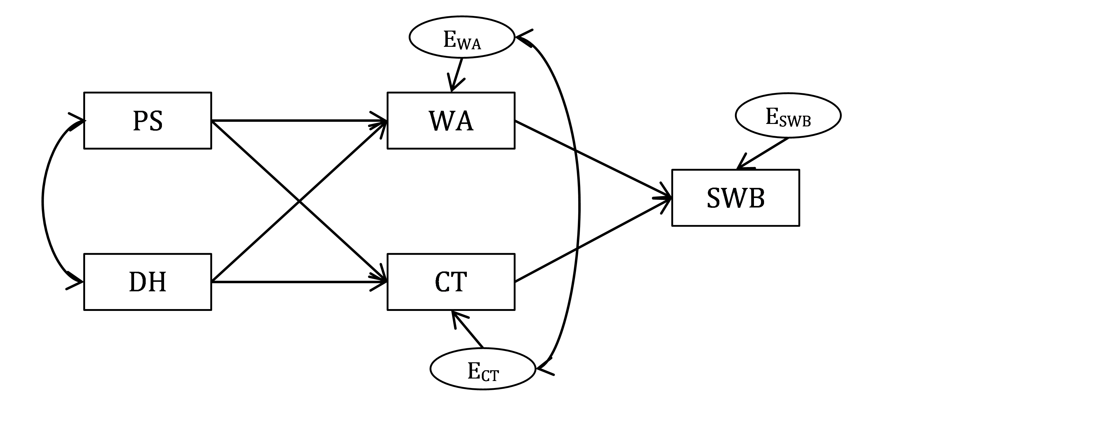
Figure 18.1: Bottom-up model of Well-being.
QUESTION 1. How many observed and latent variables are there in your model? What are the latent variables in this model? What are the exogenous and endogenous variables in this model?
Now you need to “code” this model, using the lavaan syntax conventions.To describe the model in Figure 18.1 in words, we need to mention all of its regression relationships. Let’s work from left to right of the diagram:
• WA is regressed on PS and DH (residual for WA is assumed)
• CT is regressed on PS and DH (residual for CT is assumed)
• SWB is regressed on WA and CT (residual for SWB is assumed)
We also need to mention all covariance relationships:
• PS is correlated with DH
• Residual for WA is correlated with residual for CT
Try to write the respective statements using the shorthand symbol ~ for is regressed on, symbol ~~ for is correlated with, and the plus sign + for and.
You should obtain something similar to this (I called my model W.model, but you can call it whatever you like):
W.model <- '
# regressions
   WA ~ PS + DH
   CT ~ PS + DH
   SWB ~ WA + CT
# covariance of IVs
   PS ~~ DH
# residual covariance of DVs
   WA ~~ CT '
NOTE that to describe covariance between residuals of WA and CT, we just referred to the variables themselves (WA ~~ CT). Actually, lavaan understands what we mean, because for DVs, variances are “written away” to their predictors, and what is left over is the residual, so by referring to the DV in a variance or covariance statement, you actually referring to its residual. In the output, you will see that lavaan acknowledges this by writing .WA ~~.CT, with dots in front of variable names to mark their residuals.
To fit this path model, we need function sem(). It works very similarly to function cfa() we used in Exercises 16 and 17 to fit CFA models. We need to pass the model description (model=W.model, or simply W.model if you put this argument first), and the data. However, we cannot specify data=Wellbeing because the argument data is reserved for raw data (subjects by variables), but our data is the correlation matrix! Instead, we need to pass our matrix to the argument sample.cov, which is reserved for sample covariance (or correlation) matrices. We also need to pass the number of observations (sample.nobs=149), because the correlations do not provide this information.
# Attention!
# We use "sample.cov=" because our data is the correlation matrix!
# Use "data=" for any standard case-by-variable data
sem(W.model, sample.cov=Wellbeing, sample.nobs=149)
That’s all you need to do to fit a scary looking path model from Figure 18.1. Simple, right?
Step 3. Assessing Goodness of Fit with global indices and residuals
If you run the above command, you will get a very basic output telling you that the model estimation ended normally, and giving you the chi-square statistic. To get access to full results, assign the results to a new object (for example, fit), and request the extended output including fit measures:
Now examine the output, starting with assessment of goodness of fit, and try to answer the following questions.
QUESTION 2. How many parameters are there to estimate? How many known pieces of information (sample moments) are there in the data? What are the degrees of freedom and how are they calculated?
QUESTION 3. Interpret the chi-square. Do you retain or reject the model?
Now consider the following. McDonald (1999) argued that “researchers appear to rely too much on goodness-of-fit indices, when the actual discrepancies [residuals] are much more informative” (p.390). He refers to indices such as RMSEA and CFI, which we used to judge the goodness of fit of CFA models. He continues: “generally, indices of fit are not informative in path analysis. This is because large parts of the model can be unrestrictive, with only a few discrepancies capable of being non-zero”.
To obtain residuals, which are differences between observed and ‘fitted’/‘reproduced’ covariances, request this additional output:
## $type
## [1] "raw"
##
## $cov
##         WA     CT    SWB     PS     DH
## WA   0.000
## CT   0.000  0.000
## SWB  0.000  0.000  0.000
## PS   0.000  0.000  0.096  0.000
## DH   0.000  0.000 -0.084  0.000  0.000
The residuals show how well the observed covariances are reproduced by the model. Since our observed covariances are actually correlations (we worked with the correlation matrix), interpretation of residuals is simple. Just think of them as differences between 2 sets of correlations. We usually interpret a correlation of 0.1 as small; and correlations below 0.1 trivial. Use the same logic for interpreting the residual correlations.
Note. In factor models, we used SRMR (standardized root mean square residual) to assess the average magnitude of the discrepancies between observed and expected covariances in the correlation metric. This summary was useful since in factor models, no direct covariances between observed variables were allowed (remember the local independence assumption?) and all these covariances needed to be reproduced by the factor model. In Path Analysis models, however, this index makes little sense because direct covariance paths are allowed and therefore the reproduced correlations for them will be exact (residuals = 0). Averaging (many) zero residuals with (few) non-zero ones will give a false impression that the model fits well. So, ALWAYS look at the individual residuals, and pay attention to those close or exceeding 0.1.
Also request standardized residuals, to formally test for significant differences from zero. Any standardized residual larger than 1.96 in magnitude (approximately 2 standard deviations from the mean in the standard normal distribution) is significantly different from 0 at p=.05 level.
## $type
## [1] "standardized"
##
## $cov
##         WA     CT    SWB     PS     DH
## WA   0.000
## CT   0.000  0.000
## SWB  0.000  0.000  0.000
## PS   0.000  0.000  2.051  0.000
## DH   0.000  0.000 -1.791  0.000  0.000
QUESTION 4. Are there any large residuals? Are there any statistically significant residuals? What can you say about the model fit based on the residuals?
We will not modify the model by adding any other paths to it – it already has only 2 degrees of freedom, and we will reduce this number further by adding parameters.
Step 4. Interpreting the parameter estimates
OK, let us now examine the full output (scroll up in the Console to see it, or call summary(fit) again). Find estimated regression paths (statements ~), variances (statements with names of variables or their residuals) and covariances (statements ~~). Try to answer the following questions.
QUESTION 5. Interpret the regression coefficients and their standard errors. Note that the observed variables in this study are standardized since we are working with the correlation matrix, so the regression paths are like ‘beta’ coefficients in regression and are easy to interpret.
QUESTION 6. Examine Variances output. Are the variances of regression residuals (.SWB, .WA and .CT) small or large, and what do you compare them to in order to judge their size?
Step 5. Computing indirect and total effects
It is sometimes important for research to quantify the effects – direct, indirect and total. In the bottom-up model of Wellbeing, we might be interested in describing the effect that Physical Symptoms (PS) have on Subjective Wellbeing (SWB). If you look on the diagram again, you will see that PS does not influence SWB directly, only indirectly via two routes – via WA and via CT. To compute each of these indirect effects, we need to multiply the path coefficients along each route. This will give us two indirect effects. To compute the total effect, we will need to add the two indirect effects via the two routes. There is nothing else to add here, because there is no other way of getting from PS to SWB.
You could do all these calculations by looking up the obtained parameter estimates and then multiplying and adding them (simple but tedious!). Or, you could actually ask lavaan to do these for you while fitting the model. To do the latter, you need to create ‘labels’ for the parameters of interest, and then write formulas with these labels (also a bit tedious, but much less room for errors!). It will be useful to learn how to create labels, because we will use them later in the course.
According to the diagram in Figure 18.2, I will label the path from PS to WA as a1 and path from WA to SWB as b1. Then, my indirect effect from PS to SWB via WA will be equal a1*b1. I will label the path from PS to CT as a2 and path from CT to SWB as b2. Then, my indirect effect from PS to SWB via CT will be equal a2*b2.
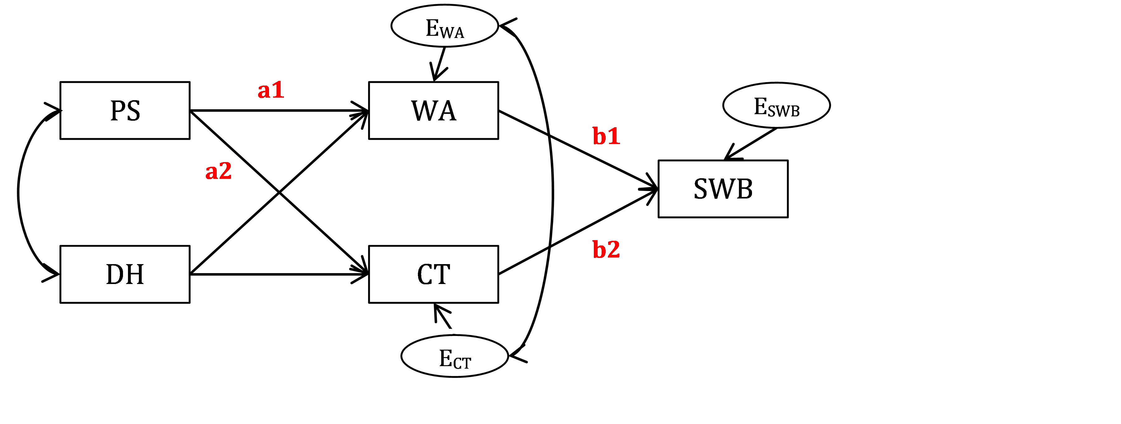
Figure 18.2: Bottom-up model of Well-being with parameter labels.
Now look how I will modify the syntax to get these labels in place, in a new model called W.model.label. The way to label a path coefficient is to add a multiplier in front of the relevant variable (predictor), as is typical for regression equations.
W.model.label <- '
# regressions - now with parameter labels assigned
   WA ~ a1*PS + DH
   CT ~ a2*PS + DH
   SWB ~ b1*WA + b2*CT
# covariance of IVs (same as before)
   PS ~~ DH
# residual covariance of DVs (same as before)
  WA ~~ CT
# Here we describe new indirect effects
   ind.WA := a1*b1    # indirect via WA
   ind.CT := a2*b2    # indirect via CT
   ind.total := ind.WA + ind.CT
'
Describe and estimate this new model and obtain the summary output. Note that the model fit or any of the existing paths will not change! This is because the model has not changed; all that we have done is assigned labels to previously “unlabeled” regression paths. But, you should see the following additions to the output. First, you should see the labels appearing next to the relevant parameters:
Regressions:
                 Estimate  Std.Err  z-value  P(>|z|)
WA ~
  PS        (a1)   -0.339    0.080   -4.256    0.000
  DH               -0.165    0.080   -2.065    0.039
CT ~
  PS        (a2)   -0.191    0.078   -2.430    0.015
  DH               -0.349    0.078   -4.452    0.000
SWB ~
  WA        (b1)    0.328    0.061    5.332    0.000
  CT        (b2)    0.550    0.061    8.950    0.000
Second, you should have a new section Defined Parameters with calculated effects:
Defined Parameters:
                 Estimate  Std.Err  z-value  P(>|z|)
  ind.WA           -0.111    0.033   -3.326    0.001
  ind.CT           -0.105    0.045   -2.345    0.019
  ind.total        -0.216    0.062   -3.463    0.001
Now you can interpret this output. (Our variables are standardized, making it easy to interpret the indirect and total effects). Try to answer the following questions.
QUESTION 7. What is the indirect effect of PS on SWB via WA? What is the indirect effect of PS on SWB via CT? What is the total indirect effect of PS on SWB (the sum of the indirect paths via WA and CT)? How do the numbers correspond to the observed covariance of PS and SWB?
Step 6. Appraising the bottom-up model of Wellbeing critically
Finally, let us critically evaluate the model. Specifically, let us think of causality in this study. The article’s abstract suggested that there was an equally plausible top-down model of subjective well-being, in which Subjective well-being causes World Assumptions and Constructive Thinking, with those in turn influencing Physical Symptoms and Daily Hassles. Path Analysis in itself cannot prove causality, so the analysis cannot tell us which model – the bottom-up or the top-down – is better. You could say: “but this study employed a longitudinal design, where subjective well-being was measured one month later than the predictor variables”. Unfortunately, even longitudinal designs cannot always disentangle the causes and effects. The fact that SWB was measured one month after the other constructs does not mean it was caused by them, because SWB was very stable over that time (the article reports test-retest correlation = 0.92), and it is therefore a good proxy for SWB at baseline, or possibly even before the baseline.
QUESTION 8 (Optional challenge). Can you try to suggest a research design that will address these problems and help establish causality in this study?
Step 7. Saving your work
After you finished work with this exercise, save your R script with a meaningful name, for example “Bottom-up model of Wellbeing”. To keep all of the created objects, which might be useful when revisiting this exercise, save your entire ‘work space’ when closing the project. Press File / Close project, and select “Save” when prompted to save your ‘Workspace image’.
18.4 Solutions
Q1. There are 8 variables in this model – 5 observed variables, and 3 unobserved variables (the 3 regression residuals). There are 5 exogenous (independent) variables: PS and DH (observed), and residuals .WA, .SWB and .CT (unobserved). There are 3 endogenous (dependent) variables: WA, CT and SWB.
Q2. The output prints that the “Number of free parameters” is 13. You can work out what these are just by looking at the diagram, or by counting the number of ‘Parameter estimates’ printed in the output. The best way to practice is to have a go just looking at the diagram, and then check with the output. There are 6 regression paths (arrows on diagram) to estimate. There are also 3 paths from residuals to the observed variables, but they are fixed to 1 for setting the scale of residuals and therefore are not estimated. There are 2 covariances (bi-directional arrows) to estimate: one for the independent variables PS and DH, and the other is for the residuals of WA and CT. There are 5 variances (look at how many IVs you have) to estimate. There are 3 variances of residuals, and also 2 variances of the independent (exogenous) variables PS and DH. In total, this makes 6+2+5=13 parameters.
Now let’s calculate sample moments, which is the number of observed variances and covariances. There are 5 observed variables, therefore 5(5+1)/2 = 15 moments in total (made up from 5 variances and 10 covariances). The degrees of freedom* is then 15 (moments) – 13 (parameters) = 2 (df).
Q3. The chi-square test (Chi-square = 10.682, Degrees of freedom = 2, P-value = .005) suggests rejecting the model because the test is significant (p-value is very low). In this case, we cannot “blame” the poor chi-square result on the large sample size (our sample is not that large).
Q4. The residual output makes it very clear that all but 2 covariances were freely estimated (and fully accounted for) by the model – this is why their residuals are exactly 0. The only omitted connections were between DH and SWB, and between PS and SWB (look at the diagram - there are no direct paths between these pairs of variables). We modelled these relationships as fully mediated by WA and CT, respectively. So, essentially, this model tests only for the absence of 2 direct effects – the rest of the model is unrestricted. The residuals for these omitted paths are small in magnitude (just under 0.1), but one borderline residual PS/SWB (=0.096) is significantly different from zero (stdz value = 2.051 is larger than the critical value 1.96).
Based on the residual output, we have detected an area of local misfit, pertaining to the lack of direct path from PS to SWB. This misfit is “small” (not “trivial”) in terms of effect size, and it is significant.
Q5. All paths are significant at the 0.05 level (p-values are less than 0.05), and the standard errors of these estimates are small (of magnitude 1/SQRT(N), as they should be for an identified model).
Regressions:
                Estimate  Std.Err  z-value  P(>|z|)
WA ~
  PS               -0.339    0.080   -4.256    0.000
  DH               -0.165    0.080   -2.065    0.039
CT ~
  PS               -0.191    0.078   -2.430    0.015
  DH               -0.349    0.078   -4.452    0.000
SWB ~
  WA                0.328    0.061    5.332    0.000
  CT                0.550    0.061    8.950    0.000
Q6. Considering that all our observed variables have variance 1, the variances for residuals .WA and .CT are quite large (about 0.8). So the predictors only explained about 20% of variance in these variables. The error variance for .SWB is quite small (0.39) – which means that the majority of variance in SWB is explained by the other variables in the model.
Variances:
                Estimate  Std.Err  z-value  P(>|z|)
.WA                0.811    0.094    8.631    0.000
.CT                0.787    0.091    8.631    0.000
.SWB               0.390    0.045    8.631    0.000
Q7. The total indirect effect of PS on SWB is –.216. Let’s see how it is computed. Look at the regression weights in the answer to Q5. The route from PS to SWB via WA: (–0.339)0.328=–0.111. The route from PS to SWB via CT: (–0.191)0.550=–0.105. Adding these two routes, we get the indirect effect = –0.216. This shows you how to compute the effects from given parameter values by hand, but we obtained the same answers through parameter labels.
Now, if you look into the original correlation matrix, View(Wellbeing), you will see that the covariance of PS and SWB is -0.21. This is close to the total indirect effect (-0.216). The values are not exactly the same, which means that the indirect effects do not explain the observed covariance fully. Adding a direct path from PS to SWB (which is omitted in this model) would explain the observed covariance 100%.
Q8. Perhaps one could alter the level of daily hassles or physical symptoms through an intervention and see what difference (if any) this makes to the outcomes compared to the non-intervention condition.