Exercise 17 CFA of a correlation matrix of subtest scores from an ability test battery

Data file	Thurstone.csv
R package	lavaan

17.1 Objectives

In this exercise, you will fit a Confirmatory Factor Analysis (CFA) model, or measurement model, to a published correlation matrix of scores on subtests from an ability test battery. We already considered an Exploratory Factor Analysis (EFA) of these same data in Exercise 10. In the process of fitting a CFA model, you will start getting familiar with the SEM language and build on the techniques introduced in Exercise 16 using R package lavaan (stands for latent variable analysis).

17.2 Study of “primary mental abilities” of Louis Thurstone

This is a classic study of “primary mental abilities” by Louis Thurstone. Thurstone analysed 9 subtests, each measuring some specific mental ability with several tasks. The 9 subtests were designed to measure 3 broader mental abilities, namely:

Verbal Ability	Word Fluency	Reasoning Ability
1. sentences	4. first letters	7. letter series
2. vocabulary	5. four-letter words	8. pedigrees
3. sentence completion	6. suffixes	9. letter grouping

Each subtest was scored as a number of correctly completed tasks, and the scores on each of the 9 subtests can be considered continuous.

You will work with the published correlations between the 9 subtests, based on N=215 subjects (Thurstone, 1947). Despite having no access to the actual subject scores, the correlation matrix is all you need to fit a basic CFA model without intercepts.

17.3 Worked Example - CFA of Thurstone’s primary ability data

To complete this exercise, you need to repeat the analysis from a worked example below, and answer some questions.

Step 1. Reading and examining data

The data (subscale correlations) are stored in a comma-separated (.csv) file Thurstone.csv. If you have completed Exercise 10, you would have already downloaded this file and created a project associated with it. You can continue working in that project.

If you have not completed Exercise 10, you can download the file now into a new folder and create a project associated with it. Preview the file by clicking on Thurstone.csv in the Files tab in RStudio, and selecting View File. This will not import the data yet, just open the actual .csv file. You will see that the first row contains the subscale names - “s1”, “s2”, “s3”, etc., and the first entry in each row is again the facet names. To import this correlation matrix into RStudio preserving all these facet names for each row and each column, we will use function read.csv(). We will say that we have headers (header=TRUE), and that the row names are contained in the first column (row.names=1).

Thurstone <- read.csv(file="Thurstone.csv", header=TRUE, row.names=1)

Examine object Thurstone that should now be in the Environment tab. Examine the object by either pressing on it, or calling function View(). You will see that it is a correlation matrix, with values 1 on the diagonal, and moderate to large positive values off the diagonal. This is typical for ability tests – they tend to correlate positively with each other.

Step 2. Specifying and fitting a measurement model

Before you start using commands from the package lavaan, make sure you have it installed (if not, use menu Tools and then Install packages…), and load it:

library(lavaan)

Given that the subtests were designed to measure 3 broader mental abilities (Verbal, Word Fluency and Reasoning Ability), we will test the below CFA model.

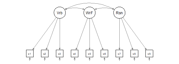
Figure 17.1: Theoretical model for Thurstone’s ability data (Verbal= Vrb, Word Fluency = WrF and Reasoning Ability = Rsn).

We need to “code” this model in syntax, using the lavaan syntax conventions. Here are these conventions:

formula type	operator	mnemonic
latent variable definition	=~	is measured by
regression	~	is regressed on
(residual) (co)variance	~~	is correlated with
intercept	~ 1	intercept

To describe the model in Figure 17.1 in words, we would say:

• Verbal is measured by s1 and s2 and s3

• WordFluency is measured by s4 and s5 and s6

• Reasoning is measured by s7 and s8 and s9

A shorthand for and is the plus sign +. So, this is how we translate the above sentences into syntax for our model (let’s call it T.model):

T.model <- ' Verbal =~ s1 + s2 + s3
             WordFluency =~ s4 + s5 + s6
             Reasoning =~ s7 + s8 + s9 '

Be sure to have the single quotation marks opening and closing the syntax. Begin each equation on the new line. Spaces within each equation are optional, they just make reading easier for you (but R does not mind).

By default, lavaan will scale each factor by setting the same unit as its first indicator (and the factor variance is then freely estimated). So, it will set the loading of s1 to 1 to scale factor Verbal, it will set the loading of s4 to 1 to scale factor WordFluency, and the loading of s7 to 1 to scale factor Reasoning. You can see this on the diagram, where the loading paths for these three indicators are in dashed rather than solid lines.

Write the above syntax in your Script, and run it by highlighting the whole lot and pressing the Run button or Ctrl+Enter keys. You should see a new object T.model appear on the Environment tab. This object contains the model syntax.

To fit this CFA model, we need function cfa(). We need to pass to this function the model name (model=T.model), and the data. However, you cannot specify data=Thurstone because the argument data is reserved for raw data (subjects x variables), but our data is the correlation matrix! Instead, we need to pass our matrix to the argument sample.cov, which is reserved for sample covariance (or correlation) matrices. [That also means that we need to convert Thurstone, which is a data frame, into matrix before submitting it to analysis.] Of course we also need to tell R the number of observations (sample.nobs=215), because the correlation matrix does not provide such information.

# convert data frame to matrix
Thurstone <- as.matrix(Thurstone)

# fit the model with default scaling, and ask for summary output 
fit <- cfa(model=T.model, sample.cov=Thurstone, sample.nobs=215)

summary(fit)

## lavaan 0.6-19 ended normally after 30 iterations
## 
##   Estimator                                         ML
##   Optimization method                           NLMINB
##   Number of model parameters                        21
## 
##   Number of observations                           215
## 
## Model Test User Model:
##                                                       
##   Test statistic                                38.737
##   Degrees of freedom                                24
##   P-value (Chi-square)                           0.029
## 
## Parameter Estimates:
## 
##   Standard errors                             Standard
##   Information                                 Expected
##   Information saturated (h1) model          Structured
## 
## Latent Variables:
##                    Estimate  Std.Err  z-value  P(>|z|)
##   Verbal =~                                           
##     s1                1.000                           
##     s2                1.010    0.050   20.031    0.000
##     s3                0.946    0.053   17.726    0.000
##   WordFluency =~                                      
##     s4                1.000                           
##     s5                0.954    0.081   11.722    0.000
##     s6                0.841    0.081   10.374    0.000
##   Reasoning =~                                        
##     s7                1.000                           
##     s8                0.922    0.097    9.514    0.000
##     s9                0.901    0.097    9.332    0.000
## 
## Covariances:
##                    Estimate  Std.Err  z-value  P(>|z|)
##   Verbal ~~                                           
##     WordFluency       0.484    0.071    6.783    0.000
##     Reasoning         0.471    0.070    6.685    0.000
##   WordFluency ~~                                      
##     Reasoning         0.414    0.067    6.147    0.000
## 
## Variances:
##                    Estimate  Std.Err  z-value  P(>|z|)
##    .s1                0.181    0.028    6.418    0.000
##    .s2                0.164    0.027    5.981    0.000
##    .s3                0.266    0.033    8.063    0.000
##    .s4                0.300    0.050    5.951    0.000
##    .s5                0.363    0.052    6.974    0.000
##    .s6                0.504    0.059    8.553    0.000
##    .s7                0.389    0.059    6.625    0.000
##    .s8                0.479    0.062    7.788    0.000
##    .s9                0.503    0.063    8.032    0.000
##     Verbal            0.815    0.097    8.402    0.000
##     WordFluency       0.695    0.100    6.924    0.000
##     Reasoning         0.607    0.099    6.115    0.000

Examine the output. Start with finding estimated factor loadings (under Latent Variables: find statements =~), factor variances (under Variances: find factor names) and covariances (under Covariances: find statements ~~).

QUESTION 1. Why are the factor loadings of s1, s4 and s7 equal 1, and no Standard Errors, z-values or p-values are printed for them? How many factor loadings are there to estimate?

QUESTION 2. How many latent variables are there in your model? What are they? What parameters are estimated for these variables? [HINT. You do not need the R output to answer the first part of the question. You need the model diagram.]

QUESTION 3. How many parameters are there to estimate in total? What are they?

QUESTION 4. How many known pieces of information (sample moments) are there in the data? What are the degrees of freedom and how are they made up?

QUESTION 5. Interpret the chi-square (reported as Test statistic). Do you retain or reject the model?

To obtain more measures of fit beyond the chi-square, request an extended output:

summary(fit, fit.measures=TRUE)

QUESTION 6. Examine the extended output; find and interpret the SRMR, CFI and RMSEA.

Step 3. Alternative scaling of latent factors

Now, I suggest you change the way your factors are scaled – for the sake of learning alternative ways of scaling latent variables, which will be useful in different situations. The other popular way of scaling common factors is by setting their variances to 1 and freeing all the factor loadings.

You can use your T.model, but request the cfa() function to standardize all the latent variables (std.lv=TRUE), so that their variances are set to 1. Assign this new model run to a new object, fit.2, so you can compare it to the previous run, fit.

fit.2 <- cfa(T.model, sample.cov=Thurstone, sample.nobs=215, std.lv=TRUE)

summary(fit.2)

Examine the output. First, compare the test statistic (chi-square) between fit.2 and fit (see your answer for Q5). The two chi-square statistics and their degrees of freedom should be exactly the same! This is because alternative ways of scaling do not change the model fit or the number of parameters. They just swap the parameters to be estimated. The standardized version of T.model sets the factor variances to 1 and estimates all factor loadings, while the original version sets 3 factor loadings (one per each factor) to 1 and estimates 3 factor variances. The difference between the two models is the matter of scaling - otherwise they are mathematically equivalent. This is nice to know, so you can use one or the other way of scaling depending on what is more convenient in a particular situation.

Step 4. Interpreting model parameters

OK, now examine the latest output with standardized latent variables (factors), interpret its parameters and answer the following questions.

QUESTION 7. Interpret the factor loadings and their standard errors.

QUESTION 8. Interpret factor covariances. Are they what you would expect?

QUESTION 9. Are the error variances small or large, and what do you compare them to in order to judge their magnitude?

Now obtain the standardized solution (in which EVERYTHING is standardized - the latent and observed variables) by adding standardized=TRUE to the summary() output:

summary(fit.2, standardized=TRUE)

QUESTION 10. Compare the default (unstandardized) parameter values in Estimate column, values in Std.lv column (standardized on latent variables only), and values in Std.all column (standardized on all - latent and observed variables). Can you explain why Estimate are identical to Std.lv, and Std.all are nearly identical to them both?

Step 5. Examining residuals and local areas of misfit

Now request two additional outputs – fitted covariance matrix and residuals. The fitted covariances are covariances predicted by the model. Residuals are differences between fitted and actual observed covariances.

fitted(fit.2)

## $cov
##       s1    s2    s3    s4    s5    s6    s7    s8    s9
## s1 0.995                                                
## s2 0.823 0.995                                          
## s3 0.771 0.779 0.995                                    
## s4 0.484 0.489 0.458 0.995                              
## s5 0.461 0.466 0.437 0.663 0.995                        
## s6 0.407 0.411 0.385 0.584 0.557 0.995                  
## s7 0.471 0.476 0.446 0.414 0.395 0.348 0.995            
## s8 0.435 0.439 0.411 0.382 0.364 0.321 0.560 0.995      
## s9 0.424 0.429 0.402 0.373 0.356 0.313 0.547 0.504 0.995

residuals(fit.2)

## $type
## [1] "raw"
## 
## $cov
##        s1     s2     s3     s4     s5     s6     s7     s8     s9
## s1  0.000                                                        
## s2  0.001  0.000                                                 
## s3  0.001 -0.003  0.000                                          
## s4 -0.047  0.002  0.000  0.000                                   
## s5 -0.031 -0.004 -0.014  0.008  0.000                            
## s6  0.038  0.076  0.056  0.003 -0.019  0.000                     
## s7 -0.026 -0.046 -0.047 -0.035  0.005 -0.061  0.000              
## s8  0.104  0.096  0.120 -0.033  0.001 -0.002 -0.007  0.000       
## s9 -0.046 -0.072 -0.044  0.049  0.088  0.010  0.048 -0.054  0.000

Examine the fitted covariances and compare them to the observed covariances for the 9 subtests - you can see them again by calling View(Thurstone).

The residuals show if all covariances are well reproduced by the model. Since our observed covariances are actually correlations (we worked with correlation matrix, with 1 on the diagonal), interpretation of residuals is very simple. Just think of them as differences between 2 sets of correlations, with the usual effect sizes assumed for correlation coefficients.

You can also request standardized residuals, to formally test for significant differences from zero. Any standardized residual larger than 1.96 in magnitude (approximately 2 standard deviations from the mean in the standard normal distribution) is significantly different from 0 at p=.05 level.

residuals(fit.2, type="standardized")

QUESTION 11. Are there any large residuals? Are there any statistically significant residuals?

Now request modification indices by calling

modindices(fit.2)

QUESTION 12. Examine the modification indices output. Find the largest index. What does it suggest?

Step 6. Modifying the model

Modify the model by adding a direct path from Verbal factor to subtest 8 (allow s8 to load on the Verbal factor). All you need to do is to add the indicator s8 to the definition of the Verbal factor in T.model, creating T.model.m:

T.model.m <- ' Verbal =~ s1+s2+s3 + s8
               WordFluency =~ s4+s5+s6
               Reasoning =~ s7+s8+s9 '

Re-estimate the modified model following the steps as with T.model, and assign the results to a new object fit.m.

QUESTION 13. Examine the modified model summary output. What is the chi-square for this modified model? How many degrees of freedom do we have and why? Do we accept or reject this modified model?

Step 7. Saving your work

After you finished work with this exercise, save your R script by pressing the Save icon in the script window. To keep all the created objects (such as fit.2), which might be useful when revisiting this exercise, save your entire work space. To do that, when closing the project by pressing File / Close project, make sure you select Save when prompted to save your “Workspace image”.

17.4 Solutions

Q1. Factor loadings for s1, s4 and s7 were not actually estimated; instead, they were fixed to 1 to set the scale of the latent factors (latent factors then simply take the scale of these particular measured variables). That is why there is no usual estimation statistics reported for these. Factor loadings for the remaining 6 subtests (9-3=6) are free parameters in the model to estimate.

Q2. There are 12 unobserved (latent) variables – 3 common factors (Verbal, WordFluency and Reasoning), and 9 unique factors /errors (these are labelled by the prefix . in front of the observed variable to which this error term is attached, for example .s1, .s2, etc. It so happens that in this model, all the latent variables are exogenous (independent), and for that reason variances for them are estimated. In addition, covariances are estimated between the 3 common factors (3 covariances, one for each pair of factors). Of course, the errors are assumed uncorrelated (remember the local independence assumption in factor analysis?), and so their covariances are fixed to 0 (not estimated and not printed in the output).

Q3. You can look this up in lavaan output. It says: Number of free parameters 21. To work out how this number is derived, you can look how many rows of values are printed in Parameter Estimates under each category. The model estimates: 6 factor loadings (see Q1) + 3 factor variances (see Q2) + 3 factor covariances (see Q2) + 9 error variances (see Q2). That’s it. So we have 6+3+3+9=21 parameters.

Q4. Sample moments refers to the number of variances and covariances in our observed data. To know how many sample moments there are, the only thing you need to know is how many observed variables there are. There are 9 observed variables, therefore there are 9 variances and 9(9-1)/2=36 covariances, 45 “moments” in total.
[Since our data is the correlation matrix, these sample moments are actually right in front of you. How many unique cells are in the 9x9 correlation matrix? There are 81 cells, but not all of them are unique, because the top and bottom off-diagonal parts are mirror images of each other. So, we only need to count the diagonal cells and the top off-diagonal cells, 9 + 36 = 45. ]

You can use the following formula for calculating the number of sample moments for any given data: m(m+1)/2 where m is the number of observed variables.

Q5. Chi-square is 38.737 (df=24). We have to reject the model, because the test indicates that the probability of this factor model holding in the population is less than .05 (P = .029).

Q6. Comparative Fit Index (CFI) = 0.986, which is larger than 0.95, indicating excellent fit. The Root Mean Square Error of Approximation (RMSEA) = 0.053, just outside of the cut-off .05 for close fit. The 90% confidence interval for RMSEA is (0.017, 0.083), which just includes the cut-off 0.08 for adequate fit. Overall, RMSEA indicates adequate fit. Standardized Root Mean Square Residual (SRMR) = 0.044 is small as we would hope for a well-fitting model. All indices indicate close fit of this model, despite the significant chi-square.

Q7. All factor loadings are positive as would be expected with ability variables, since ability subtests should be positive indicators of the ability domains. The SEs are low (magnitude of 1/sqrt(N), as they should be in a properly identified model). All factor loadings are significantly different from 0 (p-values are very small).

Latent Variables:
                Estimate  Std.Err  z-value  P(>|z|)
Verbal =~                                           
  s1                0.903    0.054   16.805    0.000
  s2                0.912    0.053   17.084    0.000
  s3                0.854    0.056   15.389    0.000
WordFluency =~                                      
  s4                0.834    0.060   13.847    0.000
  s5                0.795    0.061   12.998    0.000
  s6                0.701    0.064   11.012    0.000
Reasoning =~                                        
  s7                0.779    0.064   12.230    0.000
  s8                0.718    0.065   11.050    0.000
  s9                0.702    0.065   10.729    0.000

Q8. The factor covariances are easy to interpret in terms of size, because we set the factors’ variances =1, and therefore factor covariances are correlations. The correlations between the 3 ability domains are positive and large, as expected.

Covariances:
                 Estimate  Std.Err  z-value  P(>|z|)
Verbal ~~                                           
  WordFluency       0.643    0.050   12.815    0.000
  Reasoning         0.670    0.051   13.215    0.000
WordFluency ~~                                      
  Reasoning         0.637    0.058   10.951    0.000

Q9. The error variances are certainly quite small – considering that the observed variables had variance 1 (remember, we analysed the correlation matrix, with 1 on the diagonal?), the error variance is less than half that for most subtests. The remaining proportion of variance is due to the common factors. For example, for s1, error variance is 0.18 and this means 18% of variance is due to error and the remaining 82% (1-0.18) is due to the common factors.

Variances:
                Estimate  Std.Err  z-value  P(>|z|)
.s1                0.181    0.028    6.418    0.000
.s2                0.164    0.027    5.981    0.000
.s3                0.266    0.033    8.063    0.000
.s4                0.300    0.050    5.951    0.000
.s5                0.363    0.052    6.974    0.000
.s6                0.504    0.059    8.553    0.000
.s7                0.389    0.059    6.625    0.000
.s8                0.479    0.062    7.788    0.000
.s9                0.503    0.063    8.032    0.000

Q10. The Estimate and Std.lav parameter values are identical because in fit.2, the factors were scaled by setting their variances =1. So, the model is already standardized on the latent variables (factors). The Estimate and Std.all parameter values are almost identical (allowing for the rounding error in third decimal place) because the observed variables were already standardized since we worked with a correlation matrix!

Q11. The largest residual is for correlation between s3 and s8 (.120). It is also significantly different from zero (standardized residual is 3.334, which is greater than 1.96).

Q12.

modindices(fit.2)

##            lhs op rhs     mi    epc sepc.lv sepc.all sepc.nox
## 25      Verbal =~  s4  1.030 -0.089  -0.089   -0.090   -0.090
## 26      Verbal =~  s5  0.512 -0.061  -0.061   -0.061   -0.061
## 27      Verbal =~  s6  3.764  0.162   0.162    0.163    0.163
## 28      Verbal =~  s7  5.081 -0.238  -0.238   -0.238   -0.238
## 29      Verbal =~  s8 19.943  0.447   0.447    0.448    0.448
## 30      Verbal =~  s9  4.736 -0.215  -0.215   -0.216   -0.216
## 31 WordFluency =~  s1  2.061 -0.085  -0.085   -0.085   -0.085
## 32 WordFluency =~  s2  1.158  0.063   0.063    0.064    0.064
## 33 WordFluency =~  s3  0.148  0.024   0.024    0.024    0.024
## 34 WordFluency =~  s7  2.629 -0.167  -0.167   -0.167   -0.167
## 35 WordFluency =~  s8  0.011 -0.011  -0.011   -0.011   -0.011
## 36 WordFluency =~  s9  3.341  0.180   0.180    0.180    0.180
## 37   Reasoning =~  s1  0.105  0.021   0.021    0.021    0.021
## 38   Reasoning =~  s2  0.341 -0.038  -0.038   -0.038   -0.038
## 39   Reasoning =~  s3  0.089  0.021   0.021    0.021    0.021
## 40   Reasoning =~  s4  0.626 -0.076  -0.076   -0.076   -0.076
## 41   Reasoning =~  s5  1.415  0.111   0.111    0.111    0.111
## 42   Reasoning =~  s6  0.182 -0.039  -0.039   -0.039   -0.039
## 43          s1 ~~  s2  0.164  0.018   0.018    0.105    0.105
## 44          s1 ~~  s3  0.063  0.009   0.009    0.043    0.043
## 45          s1 ~~  s4  2.120 -0.035  -0.035   -0.150   -0.150
## 46          s1 ~~  s5  0.041 -0.005  -0.005   -0.019   -0.019
## 47          s1 ~~  s6  0.051  0.006   0.006    0.020    0.020
## 48          s1 ~~  s7  0.189  0.011   0.011    0.043    0.043
## 49          s1 ~~  s8  0.580  0.021   0.021    0.071    0.071
## 50          s1 ~~  s9  0.033 -0.005  -0.005   -0.017   -0.017
## 51          s2 ~~  s3  0.385 -0.024  -0.024   -0.114   -0.114
## 52          s2 ~~  s4  0.285  0.013   0.013    0.057    0.057
## 53          s2 ~~  s5  0.044 -0.005  -0.005   -0.021   -0.021
## 54          s2 ~~  s6  1.337  0.031   0.031    0.107    0.107
## 55          s2 ~~  s7  0.213 -0.012  -0.012   -0.047   -0.047
## 56          s2 ~~  s8  0.532  0.020   0.020    0.070    0.070
## 57          s2 ~~  s9  2.161 -0.040  -0.040   -0.140   -0.140
## 58          s3 ~~  s4  0.295  0.014   0.014    0.051    0.051
## 59          s3 ~~  s5  0.211 -0.013  -0.013   -0.041   -0.041
## 60          s3 ~~  s6  0.047  0.007   0.007    0.018    0.018
## 61          s3 ~~  s7  1.165 -0.031  -0.031   -0.098   -0.098
## 62          s3 ~~  s8  2.617  0.049   0.049    0.138    0.138
## 63          s3 ~~  s9  0.043 -0.006  -0.006   -0.017   -0.017
## 64          s4 ~~  s5  0.985  0.065   0.065    0.196    0.196
## 65          s4 ~~  s6  0.046  0.011   0.011    0.029    0.029
## 66          s4 ~~  s7  0.015 -0.004  -0.004   -0.013   -0.013
## 67          s4 ~~  s8  1.557 -0.045  -0.045   -0.119   -0.119
## 68          s4 ~~  s9  1.193  0.040   0.040    0.103    0.103
## 69          s5 ~~  s6  1.275 -0.057  -0.057   -0.134   -0.134
## 70          s5 ~~  s7  0.380  0.022   0.022    0.059    0.059
## 71          s5 ~~  s8  0.322 -0.021  -0.021   -0.051   -0.051
## 72          s5 ~~  s9  2.937  0.065   0.065    0.151    0.151
## 73          s6 ~~  s7  1.963 -0.054  -0.054   -0.123   -0.123
## 74          s6 ~~  s8  0.066  0.010   0.010    0.021    0.021
## 75          s6 ~~  s9  0.201 -0.018  -0.018   -0.037   -0.037
## 76          s7 ~~  s8  0.257 -0.031  -0.031   -0.071   -0.071
## 77          s7 ~~  s9  9.757  0.183   0.183    0.414    0.414
## 78          s8 ~~  s9  6.840 -0.141  -0.141   -0.287   -0.287

The largest index is for the factor loading Verbal =~ s8 (19.943). It is at least twice larger than any other indices. This means that chi-square would reduce by at least 19.943 if we allowed subtest s8 to load on the Verbal factor (note that currently it does not, because only s1, s2 and s3 load on Verbal). It appears that solving subtest 8 (“Pedigrees” - Identification of familial relationships within a family tree) requires verbal as well as reasoning ability (s8 is factorially complex).

Q13.

# fit the model with default scaling, and ask for summary output 
fit.m <- cfa(model=T.model.m, sample.cov=Thurstone, sample.nobs=215)
summary(fit.m)

For the modified model, Chi-square = 20.882, Degrees of freedom = 23, p-value = .588. The number of DF is 23, not 24 as in the original model. This is because we added one more parameter to estimate (factor loading), therefore losing 1 degree of freedom. The model fits the data (the p-value is insignificant), and we accept it.