Exercise 16 CFA of polytomous item scores
| Data file | CHI_ESQ2.txt |
| R package | lavaan |
16.1 Objectives
In this exercise, you will fit a Confirmatory Factor Analysis (CFA) model, or measurement model, to polytomous responses to a short service satisfaction questionnaire. We already established a factor structure for this questionnaire using Exploratory Factor Analysis (EFA) in Exercise 9. This time, we will confirm this structure using CFA. However, we will confirm it on a different sample from the one we used for EFA.
In the process of fitting a CFA model, you will start getting familiar with the SEM language and techniques using R package lavaan (stands for latent variable analysis).
16.2 Study of service satisfaction using Experience of Service Questionnaire (CHI-ESQ)
In 2002, Commission for Health Improvement in the UK developed the Experience of Service Questionnaire (CHI-ESQ) to measure user experiences with the Child and Adolescent Mental Health Services (CAMHS). The questionnaire exists in two versions: one for older children and adolescents for describing experiences with their own treatment, and the other is for parents/carers of children who underwent treatment. We will consider the version for parents/carers.
The CHI-ESQ parent version consists of 12 questions covering different types of experiences. Here are the questions:
1. I feel that the people who have seen my child listened to me
2. It was easy to talk to the people who have seen my child
3. I was treated well by the people who have seen my child
4. My views and worries were taken seriously
5. I feel the people here know how to help with the problem I came for
6. I have been given enough explanation about the help available here
7. I feel that the people who have seen my child are working together
   to help with the problem(s)
8. The facilities here are comfortable (e.g. waiting area)
9. The appointments are usually at a convenient time (e.g. don’t
   interfere with work, school)
10. It is quite easy to get to the place where the appointments are
11. If a friend needed similar help, I would recommend that he or she
    come here
12. Overall, the help I have received here is good
Parents/carers are asked to respond to these questions using response options “Certainly True” — “Partly True” — “Not True” (coded 1-2-3) and Don’t know (not scored but treated as missing data, “NA”). Note that there are quite a lot of missing responses!
Participants in this study are N=460 parents reporting on experiences with one CAMHS member Service. This is a subset of the large multi-service sample analysed and reported in Brown, Ford, Deighton, & Wolpert (2014), and, importantly, these data are from a different member service than the data we considered in Exercise 9.
16.3 Worked Example - CFA of responses to CHI-ESQ parental version
To complete this exercise, you need to repeat the analysis from a worked example below, and answer some questions.
Step 1. Importing and examining the data
The data are stored in the space-separated (.txt) file CHI_ESQ2.txt. Download the file now into a new folder and create a project associated with it. Preview the file by clicking on CHI_ESQ2.txt in the Files tab in RStudio (this will not import the data yet, just open the actual file). You will see that the first row contains the item abbreviations (esq+p for “parent”): “esqp_01”, “esqp_02”, “esqp_03”, etc., and the first entry in each row is the respondent number: “1”, “2”, …“620”. Function read.table() will import this into RStudio taking care of these column and row names. It will actually understand that we have headers and row names because the first row contains one fewer fields than the number of columns (see ?read.table for detailed help on this function).
We have just read the data into a new data frame named CHI_ESQ2. Examine the data frame by either pressing on it in the Environment tab, or calling function View(CHI_ESQ2). You will see that there are quite a few missing responses, which could have occurred because either “Don’t know” response option was chosen, or because the question was not answered at all.
Step 2. Specifying and fitting a measurement model
Before you start using commands from the package lavaan, make sure you have it installed (if not, use menu Tools and then Install packages…), and load it.
Given that we already established the factor structure for CHI-ESQ by the means of EFA in Exercise 9, we will fit a model with 2 correlated factors - Satisfaction with Care (Care for short) and Satisfaction with Environment (Environment for short).
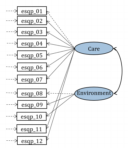
Figure 16.1: Confirmatory model for CHI-ESQ (paths fixed to 1 are in dashed lines).
We need to “code” this model in syntax, using the lavaan syntax conventions. Here are these conventions:
| formula type | operator | mnemonic |
|---|---|---|
| latent variable definition | =~ | is measured by |
| regression | ~ | is regressed on |
| (residual) (co)variance | ~~ | is correlated with |
| intercept | ~ 1 | intercept |
To describe the model in Figure 16.1 in words, we would say:
• Care is measured by esqp_01 and esqp_02 <…> and esqp_11 and esqp_12
• Environment is measured by esqp_08 and esqp_09 and esqp_10
A shorthand for and is the plus sign +. So, this is how we translate the above sentences into syntax for our model (let’s call it ESQmodel):
ESQmodel <- 'Care =~ esqp_01+esqp_02+esqp_03+esqp_04+
                     esqp_05+esqp_06+esqp_07+
                     esqp_11+esqp_12
             Environment =~ esqp_08+esqp_09+esqp_10 '
Be sure to have the single quotation marks opening and closing the syntax. Begin each equation on a new line. Spaces within each equation are optional, they just make reading easier for you (but R does not mind).
By default, lavaan will scale each factor by setting the same unit as its first indicator (and the factor variance is then freely estimated). So, it will set the loading of esqp_01 to 1 to scale factor Care, it will set the loading of esqp_08 to 1 to scale factor Environment. You can see this on the diagram, where the loading paths for these three indicators are in dashed rather than solid lines.
Write the above syntax in your Script, and run it by highlighting the whole lot and pressing the Run button or Ctrl+Enter keys. You should see a new object ESQmodel appear on the Environment tab. This object contains the model syntax.
To fit this CFA model, we need function cfa(). We need to pass to this function the data frame CHI_ESQ2 and the model name (model=ESQmodel).
# fit the model with default scaling, and ask for summary output
fit <- cfa(model=ESQmodel, data=CHI_ESQ2)

summary(fit)
## lavaan 0.6-19 ended normally after 56 iterations
##
## Estimator ML
## Optimization method NLMINB
## Number of model parameters 25
##
## Used Total
## Number of observations 331 460
##
## Model Test User Model:
##
## Test statistic 264.573
## Degrees of freedom 53
## P-value (Chi-square) 0.000
##
## Parameter Estimates:
##
## Standard errors Standard
## Information Expected
## Information saturated (h1) model Structured
##
## Latent Variables:
## Estimate Std.Err z-value P(>|z|)
## Care =~
## esqp_01 1.000
## esqp_02 0.970 0.074 13.108 0.000
## esqp_03 0.607 0.054 11.255 0.000
## esqp_04 1.140 0.072 15.883 0.000
## esqp_05 1.441 0.090 15.979 0.000
## esqp_06 1.192 0.088 13.525 0.000
## esqp_07 1.321 0.089 14.924 0.000
## esqp_11 1.242 0.079 15.647 0.000
## esqp_12 1.270 0.076 16.620 0.000
## Environment =~
## esqp_08 1.000
## esqp_09 1.520 0.368 4.135 0.000
## esqp_10 0.921 0.227 4.050 0.000
##
## Covariances:
## Estimate Std.Err z-value P(>|z|)
## Care ~~
## Environment 0.033 0.009 3.835 0.000
##
## Variances:
## Estimate Std.Err z-value P(>|z|)
## .esqp_01 0.099 0.008 11.732 0.000
## .esqp_02 0.127 0.011 12.036 0.000
## .esqp_03 0.080 0.007 12.356 0.000
## .esqp_04 0.077 0.007 10.966 0.000
## .esqp_05 0.119 0.011 10.902 0.000
## .esqp_06 0.171 0.014 11.937 0.000
## .esqp_07 0.140 0.012 11.476 0.000
## .esqp_11 0.099 0.009 11.114 0.000
## .esqp_12 0.073 0.007 10.366 0.000
## .esqp_08 0.204 0.020 10.431 0.000
## .esqp_09 0.171 0.027 6.352 0.000
## .esqp_10 0.172 0.017 10.421 0.000
## Care 0.130 0.016 7.936 0.000
## Environment 0.045 0.016 2.809 0.005Examine the output. Start with finding estimated factor loadings (under Latent Variables: find statements =~), factor variances (under Variances: find statements ~~) and covariances (under Covariances: find statements ~~).
QUESTION 1. Why are the factor loadings of esqp_01 and esqp_08 equal to 1, and no Standard Errors, z-values or p-values are printed for them? How many factor loadings are there to estimate?
QUESTION 2. How many latent variables are there in your model? What are they? What parameters are estimated for these variables? [HINT. You do not need the R output to answer the first part of the question. You need the model diagram.]
QUESTION 3. How many parameters are there to estimate in total? What are they?
QUESTION 4. How many known pieces of information (sample moments) are there in the data? What are the degrees of freedom and how are they made up?
QUESTION 5. Interpret the chi-square (reported as Test statistic). Do you retain or reject the model?
To obtain more measures of fit beyond the chi-square, request an extended output:
QUESTION 6. Examine the extended output; find and interpret the SRMR, CFI and RMSEA.
Step 3. Alternative scaling of latent factors
Now, I suggest you change the way your factors are scaled – for the sake of learning alternative ways of scaling latent variables, which will be useful in different situations. The other popular way of scaling common factors is by setting their variances to 1 and freeing all the factor loadings.
You can use your ESQmodel, but request the cfa() function to standardize all the latent variables (std.lv=TRUE), so that their variances are set to 1. Assign this new model run to a new object, fit.2, so you can compare it to the previous run, fit.
Examine the output. First, compare the test statistic (chi-square) between fit.2 and fit (see your answer for Q5). The two chi-square statistics and their degrees of freedom should be exactly the same! This is because alternative ways of scaling do not change the model fit or the number of parameters. They just swap the parameters to be estimated. The standardized version of ESQmodel sets the factor variances to 1 and estimates all factor loadings, while the original version sets 2 factor loadings (one per each factor) to 1 and estimates 2 factor variances. The difference between the two models is the matter of scaling - otherwise they are mathematically equivalent. This is nice to know, so you can use one or the other way of scaling depending on what is more convenient in a particular situation.
Step 4. Interpreting model parameters
OK, now examine the latest output with standardized latent variables (factors), and answer the following questions.
QUESTION 7. Examine the factor loadings and their standard errors. How do you interpret these loadings compared to the model where the factors were scaled by borrowing the scale of one of their indicators?
QUESTION 8. Interpret factor correlations. Are they what you would expect? (If you did Exercise 9, you can compare this result with your estimate of factor correlations)
Now obtain the standardized solution (in which EVERYTHING is standardized - the latent and observed variables) by adding standardized=TRUE to the summary() output:
QUESTION 9. Compare the default (unstandardized) parameter values in the Estimate column, values in Std.lv column (standardized on latent variables only), and values in the Std.all column (standardized on all - latent and observed variables). Can you explain why Estimate values are identical to Std.lv, but different to Std.all?
QUESTION 10. Examine the standardized (Std.all) factor loadings. How do you interpret these loadings compared to the Std.lv values?
Examining the relative size of standardized factor loadings, we can see that the “marker” (highest loading) item for factor Care is esqp_12 (Overall help) - the same result as in EFA with “oblimin” rotation in Exercise 9. The marker item for factor Environment is esqp_08 (facilities), while in EFA the marker item was esqp_09 (appointment times).
QUESTION 11. Are the standardized error variances small or large, and how do you judge their magnitude?
Step 5. Examining residuals and local areas of misfit
Now request one additional output – residuals. Residuals are differences between fitted (or predicted by the model) covariances and the actual observed covariances. The residuals show if all covariances are well reproduced by the model. But since our data are raw responses to questionnaire items, residual covariances will be relatively difficult to interpret. So, instead of requesting residual covariances, we will request residual correlations - differences between fitted and observed correlations of item responses.
## $type
## [1] "cor.bollen"
##
## $cov
##         esq_01 esq_02 esq_03 esq_04 esq_05 esq_06 esq_07 esq_11 esq_12 esq_08
## esqp_01  0.000
## esqp_02  0.124  0.000
## esqp_03  0.080  0.115  0.000
## esqp_04  0.088  0.077  0.077  0.000
## esqp_05 -0.012 -0.024  0.012 -0.021  0.000
## esqp_06 -0.045 -0.016 -0.085 -0.047  0.017  0.000
## esqp_07  0.012 -0.068  0.000 -0.028  0.032  0.035  0.000
## esqp_11 -0.067 -0.072 -0.050 -0.023  0.008  0.019 -0.039  0.000
## esqp_12 -0.074 -0.045 -0.097 -0.031 -0.003  0.049  0.035  0.102  0.000
## esqp_08 -0.009  0.064  0.040  0.061 -0.007  0.030  0.042  0.033  0.050  0.000
## esqp_09  0.029  0.098  0.127  0.014  0.017 -0.035 -0.026  0.045 -0.060 -0.034
## esqp_10  0.006 -0.043  0.036 -0.008 -0.032 -0.137 -0.108 -0.010 -0.128  0.024
##         esq_09 esq_10
## esqp_01
## esqp_02
## esqp_03
## esqp_04
## esqp_05
## esqp_06
## esqp_07
## esqp_11
## esqp_12
## esqp_08
## esqp_09  0.000
## esqp_10  0.021  0.000
Now interpretation of residuals is very simple. Just think of them as differences between 2 sets of correlations, with the usual effect sizes assumed for correlation coefficients.
You can also request standardized residuals, to formally test for significant differences from zero. Any standardized residual larger than 1.96 in magnitude (approximately 2 standard deviations from the mean in the standard normal distribution) is significantly different from 0 at p=.05 level.
QUESTION 12. Are there any large residuals? Are there any statistically significant residuals?
Now request modification indices by calling
QUESTION 13. Examine the modification indices output. Find the largest index. What does it suggest?
Step 6. Modifying the model
Modify the model by adding a covariance path (~~) between items esqp_11 and esqp_12. All you need to do is to add a new line of code to the definition of ESQmodel by using the base R function paste(), thus creating a modified model ESQmodel.m:
Re-estimate the modified model following the steps as with ESQmodel, and assign the results to a new object fit.m.
QUESTION 14. Examine the modified model summary output. What is the chi-square for this modified model? How many degrees of freedom do we have and why? What is the goodness of fit of this modified model?
Step 7. Saving your work
After you finished work with this exercise, save your R script by pressing the Save icon in the script window. To keep all the created objects (such as fit.2), which might be useful when revisiting this exercise, save your entire work space. To do that, when closing the project by pressing File / Close project, make sure you select Save when prompted to save your “Workspace image”.
16.4 Solutions
Q1. Factor loadings for esqp_01 and esqp_08 were not actually estimated; instead, they were fixed to 1 to set the scale of the latent factors (latent factors then simply take the scale of these particular measured variables). That is why there is no usual estimation statistics reported for these. Factor loadings for the remaining 10 items (12-2=10) are free parameters in the model to estimate.
Q2. There are 14 unobserved (latent) variables – 2 common factors (Care and Environment), and 12 unique factors /errors (these are labelled by the prefix . in front of the observed variable to which this error term is attached, for example .esqp_01, .esqp_02, etc. It so happens that in this model, all the latent variables are exogenous (independent), and for that reason variances for them are estimated. In addition, covariance is estimated between the 2 common factors. Of course, the errors are assumed uncorrelated (remember the local independence assumption in factor analysis?), and so their covariances are fixed to 0 (not estimated and not printed in the output).
Q3. You can look this up in lavaan output. It says: Number of free parameters 25. To work out how this number is derived, you can look how many rows of values are printed in Parameter Estimates under each category. The model estimates:
10 factor loadings (see Q1) + 2 factor variances (see Q2) + 1 factor covariance (see Q2) + 12 error variances (see Q2). That’s it. So we have 10+2+1+12=25 parameters.
Q4. Sample moments refers to the number of variances and covariances in our observed data. To know how many sample moments there are, the only thing you need to know is how many observed variables there are. There are 12 observed variables, therefore there are 12 variances and 12(12-1)/2=66 covariances, 78 “moments” in total.
You can use the following formula for calculating the number of sample moments for any given data: m(m+1)/2 where m is the number of observed variables.
Q5. Chi-square is 264.573 (df=53, which is calculated as 78 sample moments minus 35 parameters). We have to reject the model, because the test indicates that the probability of this factor model holding in the population is less than .001.
Q6. Comparative Fit Index (CFI) = 0.903, which is larger than 0.90 but smaller than 0.95, indicating adequate fit. The Root Mean Square Error of Approximation (RMSEA) = 0.110, and the 90% confidence interval for RMSEA is (0.097, 0.123), well outside of the cut-off .08 for adequate fit. Standardized Root Mean Square Residual (SRMR) = 0.054 is small as we would hope for a well-fitting model. All indices except the RMSEA indicate acceptable fit of this model.
Q7. All factor loadings are positive as would be expected with questions being positive indicators of satisfaction. The SEs are low (magnitude of 1/sqrt(N), as they should be in a properly identified model). All factor loadings are significantly different from 0 (p-values are very small).
Latent Variables:
                   Estimate  Std.Err  z-value  P(>|z|)
  Care =~
    esqp_01           0.361    0.023   15.872    0.000
    esqp_02           0.350    0.024   14.350    0.000
    esqp_03           0.219    0.018   12.011    0.000
    esqp_04           0.412    0.023   18.269    0.000
    esqp_05           0.520    0.028   18.416    0.000
    esqp_06           0.430    0.029   14.903    0.000
    esqp_07           0.477    0.028   16.845    0.000
    esqp_11           0.448    0.025   17.911    0.000
    esqp_12           0.459    0.024   19.427    0.000
  Environment =~
    esqp_08           0.211    0.038    5.617    0.000
    esqp_09           0.321    0.045    7.189    0.000
    esqp_10           0.194    0.035    5.624    0.000
Q8. The factor covariance are easy to interpret in terms of size, because we set the factors’ variances =1, and therefore factor covariance is correlation. The correlation between Care and Environment is positive and of medium size (r = 0.438). This estimate is close to the latent factor correlation estimated in EFA in Exercise 9 (r = 0.39).
Covariances:
                   Estimate  Std.Err  z-value  P(>|z|)
  Care ~~
    Environment       0.438    0.073    6.022    0.000
Q9. The Estimate and Std.lav parameter values are identical because in fit.2, the factors were scaled by setting their variances =1. So, the model is already standardized on the latent variables (factors).
The Std.lv and Std.all parameter values are different because the observed variables were raw item responses and not standardized originally. The standardization of factors (Std.lv) does not standardize the observed variables. Only in Std.all, the observed variables are also standardized. The Std.all output makes the results comparable with EFA in Exercise 9, where all variables are standardized.
Latent Variables:
                   Estimate  Std.Err  z-value  P(>|z|)   Std.lv  Std.all
  Care =~
    esqp_01           0.361    0.023   15.872    0.000    0.361    0.755
    esqp_02           0.350    0.024   14.350    0.000    0.350    0.702
    esqp_03           0.219    0.018   12.011    0.000    0.219    0.611
    esqp_04           0.412    0.023   18.269    0.000    0.412    0.830
    esqp_05           0.520    0.028   18.416    0.000    0.520    0.834
    esqp_06           0.430    0.029   14.903    0.000    0.430    0.721
    esqp_07           0.477    0.028   16.845    0.000    0.477    0.786
    esqp_11           0.448    0.025   17.911    0.000    0.448    0.819
    esqp_12           0.459    0.024   19.427    0.000    0.459    0.862
  Environment =~
    esqp_08           0.211    0.038    5.617    0.000    0.211    0.424
    esqp_09           0.321    0.045    7.189    0.000    0.321    0.614
esqp_10 0.194 0.035 5.624 0.000 0.194 0.425Q10. The Std.all loadings are interpreted as the standardized factor loadings in EFA. In models with orthogonal factors, these loadings are equal to the correlation between the item and the factor; also, squared factor loading represents the proportion of variance explained by the factor.
Q11. The Std.all error variances range from (small) 0.256 for .esqp_12 to (quite large) 0.820 for esqp_08 and esqp_10. I judge them to be “small” or “large” considering that the observed variables are now standardized and have variance 1, the error variance is simply the proportion of 1. The remaining proportion of variance is due to the common factors. For example, for esqp_12, error variance is 0.256 and this means 25.6% of variance is due to error and the remaining 74.4% (1-0.256) is due to the common factors.
Variances:
                   Estimate  Std.Err  z-value  P(>|z|)   Std.lv  Std.all
  .esqp_01           0.099    0.008   11.732    0.000    0.099    0.431
  .esqp_02           0.127    0.011   12.036    0.000    0.127    0.508
  .esqp_03           0.080    0.007   12.356    0.000    0.080    0.626
  .esqp_04           0.077    0.007   10.966    0.000    0.077    0.312
  .esqp_05           0.119    0.011   10.902    0.000    0.119    0.305
  .esqp_06           0.171    0.014   11.937    0.000    0.171    0.480
  .esqp_07           0.140    0.012   11.476    0.000    0.140    0.382
  .esqp_11           0.099    0.009   11.114    0.000    0.099    0.329
  .esqp_12           0.073    0.007   10.366    0.000    0.073    0.256
  .esqp_08           0.204    0.020   10.431    0.000    0.204    0.820
  .esqp_09           0.171    0.027    6.352    0.000    0.171    0.623
  .esqp_10           0.172    0.017   10.421    0.000    0.172    0.820
Q12. There are a few residuals over 0.1 in size. The largest is for correlation between esqp_06 and esqp_10 (-.137). It is also significantly different from zero (standardized residual is -3.155, which is greater than 1.96). There are larger standardized residuals, for example -5.320 between esqp_01 and esqp_12.
Q13.
<snip>
92  esqp_07 ~~ esqp_12  6.374  0.017   0.017    0.171    0.171
93  esqp_07 ~~ esqp_08  0.667  0.008   0.008    0.050    0.050
94  esqp_07 ~~ esqp_09  0.784 -0.009  -0.009   -0.060   -0.060
95  esqp_07 ~~ esqp_10  3.022 -0.017  -0.017   -0.106   -0.106
96  esqp_11 ~~ esqp_12 66.449  0.048   0.048    0.571    0.571
97  esqp_11 ~~ esqp_08  0.150 -0.003  -0.003   -0.024   -0.024
98  esqp_11 ~~ esqp_09  1.016  0.009   0.009    0.070    0.070
99  esqp_11 ~~ esqp_10  1.421  0.010   0.010    0.074    0.074
100 esqp_12 ~~ esqp_08  2.555  0.012   0.012    0.102    0.102
<snip>
The largest index is for the covariance esqp_11 ~~ esqp_12 (66.449). It is more than twice larger than any other indices. This means that chi-square would reduce by at least 66 if we allowed errors of esqp_11 and esqp_12 to correlate. This means that these items share something in common beyond what the factor Care accounts for.
Q14.
# fit the model with default scaling, and ask for summary output
fit.m <- cfa(model=ESQmodel.m, CHI_ESQ2, std.lv=TRUE)
summary(fit.m)
For the modified model, Chi-square = 201.249, Degrees of freedom = 52, p< .001. The number of DF is 52, not 53 as in the original model. This is because we added one more parameter to estimate (correlated error terms), therefore losing 1 degree of freedom. The model reduced the RMSEA to 0.093 (90% CI 0.08-0.107) - still too high for an adequate fit.