Exercise 24 Measuring effect of intervention by comparing change models for control and experimental groups
| Data file | Olsson.RData |
| R package | lavaan, psych |
24.1 Objectives
The objective of this exercise is to fit a full structural model to repeated observations across two groups, where one group received an intervention between the two measurement occasions and the other did not. This model will allow testing for difference between the experimental and control group in terms of the change between the two measurement occasions. You will learn how to implement measurement invariance constraints across time and groups, which are essential to make sure that the longitudinal change can be compared across groups.
24.2 Study of training intervention to improve test performance (Olsson, 1973)
This data analysis example is adopted (and adapted) from James L. Arbuckle’s (2016) User Guide to software AMOS. Arbuckle analyses a study by Olsson (1973), who administered a battery of tests to N=213 eleven-year-old students on two occasions. In this exercise, we will focus on two tests, Synonyms and Opposites. Between the two administrations of these tests, 108 of the students (the experimental group) received training that was intended to improve performance on the tests. The other 105 students (the control group) did not receive any training. As a result of taking two tests on two occasions, each of the 213 students obtained four test scores:
| Descriptions | |
|---|---|
| pre_syn | Pretest scores on the Synonyms test |
| pre_opp | Pretest scores on the Opposites test |
| post_syn | Posttest scores on the Synonyms test |
| post_opp | Posttest scores on the Opposites test |
24.3 Worked Example - Quantifying change on a latent construct after an intervention
To complete this exercise, you need to repeat the analysis from a worked example below, and answer some questions.
Step 1. Reading and examining data
Means and covariances of these four variables are available for the experimental and control groups separately. I organised the data into objects that are ready to be used by R for analyses in this exercise. These objects are packaged into file Olsson.RData. Download this file, and save it in a new folder. In RStudio, create a new project in the folder you have just created. Start a new script.
We start from loading the data into RStudio Environment.
Three new objects should appear in your Environment: Olsson.cov - a list of 2 covariance matrices, one for experimental and one for control group; Olsson.mean - a list of two vectors containing means for the two groups; and Olsson.N - a list of two sample sizes for each group. Examine these objects by calling them like so:
## $Control
##          pre_syn pre_opp post_syn post_opp
## pre_syn   37.626  24.933   26.639   23.649
## pre_opp   24.933  34.680   24.236   27.760
## post_syn  26.639  24.236   32.013   23.565
## post_opp  23.649  27.760   23.565   33.443
##
## $Experimental
##          pre_syn pre_opp post_syn post_opp
## pre_syn   50.084  42.373   40.760   37.343
## pre_opp   42.373  49.872   36.094   40.396
## post_syn  40.760  36.094   51.237   39.890
## post_opp 37.343 40.396 39.890 53.641## $Control
## [1] 18.381 20.229 20.400 21.343
##
## $Experimental
## [1] 20.556 21.241 25.667 25.870## $Control
## [1] 105
##
## $Experimental
## [1] 108QUESTION 1. Examine the means for the control and experimental groups. Remember that the fist two means pertain to the pre-test and the last two means to the post-test. Do the means increase or decrease? Are there any visible differences between the groups? How would you (tentatively) interpret the changes?
Step 2. Fitting a basic structural model for repeated measures
Given that the two subtests - synonyms and opposites - are supposed to indicate verbal ability, we will fit the following basic longitudinal measurement model to both groups.
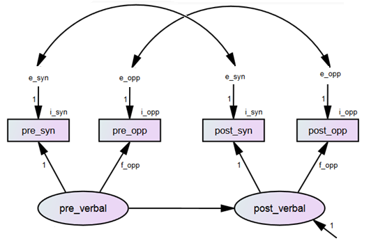
Figure 24.1: Basic model for change in verbal test performance
In this model, pre_verbal is measured by pre_syn and pre_opp, and post_verbal is measured by post_syn and post_opp. We set the factor loading of pre_syn to 1, to give the latent pre_verbal factor a unit of measurement. We set the mean of the latent pre_verbal factor to 0, to specify the origin of measurement. Because we have a repeated measures design within each group, we need to constrain measurement parameters equal across time to maintain the same scale of measurement before and after the intervention. We do so by using labels, as we did before in Exercise 22. This is regardless of any cross-group invariance considerations (which we will consider later).
The correlated unique factors (errors) for pre_syn and post_syn account for the shared variance between the Synonyms subtest on the two measurement occasions, after the verbal factor has been controlled for. The correlated unique factors (errors) for pre_opp and post_opp account for the shared variance between the Opposites subtest on the two measurement occasions, after the Verbal factor has been controlled for. This is typical for repeated measures – we have considered this feature previously in Exercise 22.
The model depicted in Figure 24.1 is the default measurement model for change that we will program in lavaan. Once we have specified this default model, we will consider how this will be implemented across groups.
Using lavaan contentions, we can specify this repeated measures model with parameter constraints (let’s call it Model.1) as follows:
Model.1 <- '
# measurement models with factor loadings equal across time  (label f_opp)
    pre_verbal =~ pre_syn + f_opp*pre_opp
    post_verbal =~ post_syn + f_opp*post_opp

# correlated residuals for repeated measures
    pre_syn ~~ post_syn
    pre_opp ~~ post_opp

# intercepts with equality constraints across time (labels i_syn and i_opp)
    pre_syn ~ i_syn*1
    post_syn ~ i_syn*1
    pre_opp ~ i_opp*1
    post_opp ~ i_opp*1

# unique factors/errors  with equality constraints across time (labels e_syn and e_opp)
    pre_syn ~~ e_syn*pre_syn
    post_syn ~~ e_syn*post_syn
    pre_opp ~~ e_opp*pre_opp
    post_opp ~~ e_opp*post_opp

# finally, the structural part (regression)
     post_verbal ~ pre_verbal '
Step 3. Setting parameters equal across groups in lavaan
Now we can deal with ensuring measurement invariance across groups. It turns out that by using the parameter equality labels in a multiple group setting, we already imposed equality constraints across the groups. This is because if a single label is attached to a parameter (say, “f_opp” was the label for factor loading of pre_opp and post_opp), then this label also holds this parameter equal across groups. if we wanted different measurement parameters across groups (but wanted to maintain longitudinal invariance) we would need to assign group-specific labels. Thankfully, we do not need to.
OK, let’s fit *thisModel.1 to both groups using sem() function of lavaan. Because our data is not a data frame with a grouping variable but instead lists of statistics for both groups, we need to specify the sample covariance matrices (sample.cov = Olsson.cov), sample means (sample.mean = Olsson.mean), and sample sizes (sample.nobs = Olsson.N). With labels set up previously to ensure invariance of repeated-measures parameters within each group, the option group.equal = c("loadings", "intercepts", "residuals") will enforce these parameters to also be invariant across groups.
library(lavaan)

fit.1 <- sem(Model.1, sample.cov = Olsson.cov, sample.mean = Olsson.mean, sample.nobs = Olsson.N,
             group.equal = c("loadings", "intercepts", "residuals"))

summary(fit.1, fit.measures=TRUE)
## lavaan 0.6-19 ended normally after 134 iterations
##
## Estimator ML
## Optimization method NLMINB
## Number of model parameters 32
## Number of equality constraints 15
##
## Number of observations per group:
## Control 105
## Experimental 108
##
## Model Test User Model:
##
## Test statistic 43.384
## Degrees of freedom 11
## P-value (Chi-square) 0.000
## Test statistic for each group:
## Control 34.035
## Experimental 9.349
##
## Model Test Baseline Model:
##
## Test statistic 689.109
## Degrees of freedom 12
## P-value 0.000
##
## User Model versus Baseline Model:
##
## Comparative Fit Index (CFI) 0.952
## Tucker-Lewis Index (TLI) 0.948
##
## Loglikelihood and Information Criteria:
##
## Loglikelihood user model (H0) -2474.985
## Loglikelihood unrestricted model (H1) -2453.294
##
## Akaike (AIC) 4983.971
## Bayesian (BIC) 5041.113
## Sample-size adjusted Bayesian (SABIC) 4987.245
##
## Root Mean Square Error of Approximation:
##
## RMSEA 0.166
## 90 Percent confidence interval - lower 0.116
## 90 Percent confidence interval - upper 0.220
## P-value H_0: RMSEA <= 0.050 0.000
## P-value H_0: RMSEA >= 0.080 0.997
##
## Standardized Root Mean Square Residual:
##
## SRMR 0.062
##
## Parameter Estimates:
##
## Standard errors Standard
## Information Expected
## Information saturated (h1) model Structured
##
##
## Group 1 [Control]:
##
## Latent Variables:
## Estimate Std.Err z-value P(>|z|)
## pre_verbal =~
## pre_syn 1.000
## pre_opp (f_pp) 0.872 0.069 12.621 0.000
## post_verbal =~
## pst_syn 1.000
## post_pp (f_pp) 0.872 0.069 12.621 0.000
##
## Regressions:
## Estimate Std.Err z-value P(>|z|)
## post_verbal ~
## pre_verbal 0.874 0.060 14.566 0.000
##
## Covariances:
## Estimate Std.Err z-value P(>|z|)
## .pre_syn ~~
## .post_syn -2.629 3.256 -0.807 0.420
## .pre_opp ~~
## .post_opp 8.412 2.763 3.045 0.002
##
## Intercepts:
## Estimate Std.Err z-value P(>|z|)
## .pre_syn (i_sy) 19.758 0.532 37.138 0.000
## .pst_syn (i_sy) 19.758 0.532 37.138 0.000
## .pre_opp (i_pp) 20.869 0.524 39.865 0.000
## .post_pp (i_pp) 20.869 0.524 39.865 0.000
##
## Variances:
## Estimate Std.Err z-value P(>|z|)
## .pre_syn (e_sy) 5.593 3.325 1.682 0.093
## .pst_syn (e_sy) 5.593 3.325 1.682 0.093
## .pre_opp (e_pp) 14.108 2.748 5.134 0.000
## .post_pp (e_pp) 14.108 2.748 5.134 0.000
## pr_vrbl 31.968 5.803 5.509 0.000
## .pst_vrb 2.841 1.643 1.729 0.084
##
##
## Group 2 [Experimental]:
##
## Latent Variables:
## Estimate Std.Err z-value P(>|z|)
## pre_verbal =~
## pre_syn 1.000
## pre_opp (f_pp) 0.872 0.069 12.621 0.000
## post_verbal =~
## pst_syn 1.000
## post_pp (f_pp) 0.872 0.069 12.621 0.000
##
## Regressions:
## Estimate Std.Err z-value P(>|z|)
## post_verbal ~
## pre_verbal 0.891 0.060 14.890 0.000
##
## Covariances:
## Estimate Std.Err z-value P(>|z|)
## .pre_syn ~~
## .post_syn 0.616 3.193 0.193 0.847
## .pre_opp ~~
## .post_opp 6.756 2.688 2.513 0.012
##
## Intercepts:
## Estimate Std.Err z-value P(>|z|)
## .pre_syn (i_sy) 19.758 0.532 37.138 0.000
## .pst_syn (i_sy) 19.758 0.532 37.138 0.000
## .pre_opp (i_pp) 20.869 0.524 39.865 0.000
## .post_pp (i_pp) 20.869 0.524 39.865 0.000
## pr_vrbl 0.714 0.862 0.828 0.407
## .pst_vrb 5.256 0.406 12.937 0.000
##
## Variances:
## Estimate Std.Err z-value P(>|z|)
## .pre_syn (e_sy) 5.593 3.325 1.682 0.093
## .pst_syn (e_sy) 5.593 3.325 1.682 0.093
## .pre_opp (e_pp) 14.108 2.748 5.134 0.000
## .post_pp (e_pp) 14.108 2.748 5.134 0.000
## pr_vrbl 45.408 7.516 6.042 0.000
## .pst_vrb 9.360 2.393 3.911 0.000Run the syntax and examine the output carefully. You should be able to see that the measurement parameters we set to be equal (factor loadings, intercepts and error variances) are indeed equal across time and also across groups.
But when examining the structural parameters, we notice that “Intercepts” for Control and Experimental groups are different. Specifically, the mean of pre_verbal is fixed at 0.000 and the intercept .post_verbal is fixed at 0.000. We know they are fixed because no Standard Errors are reported for them. This is interesting. It is common to set the origin of measurement for pre_verbal at Time 1 to 0 so that the intercepts of pre-syn and pre_opp could be estimated, but surely the intercept of post_verbal can be freely estimated given that the parameter constraints ‘pass on’ the scale of measurement from Time 1 to Time 2. However, lavaan sets the intercept of all latent factors to 0 by default. If we retain this fixed parameter, we test the following hypothesis:
Hypothsis 1 (H1). The average performance did not change across the two testing occasions in the Control group.
Initially, this appears reasonable (because the Control group did not receive any training) and we leave this intercept fixed to 0 for now.
Now, in the Experimental group, the mean of pr_verbal and the intercept of post_verbal are freely estimated (we know that because Standard Errors are reported for them), and are different from zero and from each other. Indeed, the origin and the unit of measurement can be passed on to the model for the Experimental group through the group parameter constraints. Hence, we can freely estimate the mean and variance of pre_verbal, and the intercept and residual variance of post_verbal in the Experimental group.
Now let’s examine the chi-square statistic. Chi-square for the tested model is 43.384 (df = 11); P-value < .001. We have to reject the model because the chi-square is highly significant despite the modest sample size. Because this is multiple-group analysis, the chi-square statistic is made of two group statistics: 34.035 for Control group and 9.349 for Experimental group. Clearly, the misfit comes from the Control group.
QUESTION 2. Report and interpret the SRMR, CFI and RMSEA. Would can you say about the goodness of fit of Model.1?
To help you understand the reasons for misfit, request the modification indices, and sort them from largest to smallest:
## Warning: lavaan->modindices():
##    the modindices() function ignores equality constraints; use lavTestScore()
##    to assess the impact of releasing one or multiple constraints.
## lhs op rhs block group level mi epc sepc.lv sepc.all
## 19 post_verbal ~1 1 1 1 24.972 1.631 0.312 0.312
## 18 pre_verbal ~1 1 1 1 24.972 -12.962 -2.292 -2.292
## 68 pre_syn ~~ pre_opp 2 2 1 5.936 3.732 3.732 0.420
## 71 post_syn ~~ post_opp 2 2 1 4.821 -3.363 -3.363 -0.379
## 1 pre_verbal =~ pre_syn 1 1 1 1.231 0.102 0.574 0.094
## 58 pre_syn ~~ pre_opp 1 1 1 1.087 -1.630 -1.630 -0.183
## 57 post_verbal =~ pre_opp 1 1 1 0.927 -0.085 -0.442 -0.071
## 56 post_verbal =~ pre_syn 1 1 1 0.927 0.097 0.507 0.083
## 60 pre_opp ~~ post_syn 1 1 1 0.807 1.902 1.902 0.214
## 59 pre_syn ~~ post_opp 1 1 1 0.807 -1.902 -1.902 -0.214
## 61 post_syn ~~ post_opp 1 1 1 0.636 1.248 1.248 0.140
## 20 pre_verbal =~ pre_syn 2 2 1 0.240 -0.035 -0.238 -0.033
## 65 pre_verbal =~ post_opp 2 2 1 0.192 0.029 0.195 0.028
## 64 pre_verbal =~ post_syn 2 2 1 0.192 -0.033 -0.223 -0.031
## 69 pre_syn ~~ post_opp 2 2 1 0.142 0.959 0.959 0.108
## 70 pre_opp ~~ post_syn 2 2 1 0.142 -0.959 -0.959 -0.108
## 22 post_verbal =~ post_syn 2 2 1 0.123 -0.028 -0.187 -0.026
## 67 post_verbal =~ pre_opp 2 2 1 0.040 -0.010 -0.065 -0.009
## 66 post_verbal =~ pre_syn 2 2 1 0.040 0.011 0.075 0.011
## 3 post_verbal =~ post_syn 1 1 1 0.008 -0.009 -0.048 -0.008
## 54 pre_verbal =~ post_syn 1 1 1 0.001 0.003 0.016 0.003
## 55 pre_verbal =~ post_opp 1 1 1 0.001 -0.003 -0.014 -0.002
## sepc.nox
## 19 0.312
## 18 -2.292
## 68 0.420
## 71 -0.379
## 1 0.094
## 58 -0.183
## 57 -0.071
## 56 0.083
## 60 0.214
## 59 -0.214
## 61 0.140
## 20 -0.033
## 65 0.028
## 64 -0.031
## 69 0.108
## 70 -0.108
## 22 -0.026
## 67 -0.009
## 66 0.011
## 3 -0.008
## 54 0.003
## 55 -0.002QUESTION 3. What do the modification indices tell you? Which changes in the model would produce the greatest decrease in the chi-square? How do you interpret this model change?
Step 4. Measuring change in latent factors using structural parameters in lavaan
After having answered Question 3, hopefully you agree that the lavaan defaults imposed on our structural parameters (specifically, setting the intercept of post_verbal in the Control group to 0) caused model misfit.
We will now adjust the structural model setup by freeing the intercept of post_verbal, thus allowing for change in verbal performance score between pre-test and post-test. Because the Control group did not receive any intervention, this is not “training” effect but rather “practice” effect. Modifying the model is very easy. You can just append one more line to the syntax of Model.1, explicitly freeing the intercept of post_verbal by giving it label NA, and making Model.2:
We now fit the modified model, and request summary output with fit indices and standardized parameters.
fit.2 <- sem(Model.2,
             sample.cov = Olsson.cov, sample.mean = Olsson.mean, sample.nobs = Olsson.N,
             group.equal = c("loadings", "intercepts", "residuals"))

summary(fit.2, standardized=TRUE)
## lavaan 0.6-19 ended normally after 124 iterations
##
## Estimator ML
## Optimization method NLMINB
## Number of model parameters 33
## Number of equality constraints 15
##
## Number of observations per group:
## Control 105
## Experimental 108
##
## Model Test User Model:
##
## Test statistic 14.272
## Degrees of freedom 10
## P-value (Chi-square) 0.161
## Test statistic for each group:
## Control 4.774
## Experimental 9.498
##
## Parameter Estimates:
##
## Standard errors Standard
## Information Expected
## Information saturated (h1) model Structured
##
##
## Group 1 [Control]:
##
## Latent Variables:
## Estimate Std.Err z-value P(>|z|) Std.lv Std.all
## pre_verbal =~
## pre_syn 1.000 5.642 0.937
## pre_opp (f_pp) 0.849 0.065 13.143 0.000 4.789 0.778
## post_verbal =~
## pst_syn 1.000 5.284 0.929
## post_pp (f_pp) 0.849 0.065 13.143 0.000 4.486 0.757
##
## Regressions:
## Estimate Std.Err z-value P(>|z|) Std.lv Std.all
## post_verbal ~
## pre_verbal 0.928 0.055 16.901 0.000 0.991 0.991
##
## Covariances:
## Estimate Std.Err z-value P(>|z|) Std.lv Std.all
## .pre_syn ~~
## .post_syn -3.214 3.292 -0.976 0.329 -3.214 -0.726
## .pre_opp ~~
## .post_opp 8.833 2.719 3.249 0.001 8.833 0.590
##
## Intercepts:
## Estimate Std.Err z-value P(>|z|) Std.lv Std.all
## .pre_syn (i_sy) 18.556 0.574 32.338 0.000 18.556 3.082
## .pst_syn (i_sy) 18.556 0.574 32.338 0.000 18.556 3.262
## .pre_opp (i_pp) 19.883 0.558 35.625 0.000 19.883 3.230
## .post_pp (i_pp) 19.883 0.558 35.625 0.000 19.883 3.357
## .pst_vrb 1.684 0.295 5.716 0.000 0.319 0.319
##
## Variances:
## Estimate Std.Err z-value P(>|z|) Std.lv Std.all
## .pre_syn (e_sy) 4.430 3.281 1.350 0.177 4.430 0.122
## .pst_syn (e_sy) 4.430 3.281 1.350 0.177 4.430 0.137
## .pre_opp (e_pp) 14.960 2.633 5.681 0.000 14.960 0.395
## .post_pp (e_pp) 14.960 2.633 5.681 0.000 14.960 0.426
## pr_vrbl 31.832 5.737 5.549 0.000 1.000 1.000
## .pst_vrb 0.517 1.479 0.350 0.727 0.019 0.019
##
##
## Group 2 [Experimental]:
##
## Latent Variables:
## Estimate Std.Err z-value P(>|z|) Std.lv Std.all
## pre_verbal =~
## pre_syn 1.000 6.800 0.955
## pre_opp (f_pp) 0.849 0.065 13.143 0.000 5.773 0.831
## post_verbal =~
## pst_syn 1.000 6.810 0.955
## post_pp (f_pp) 0.849 0.065 13.143 0.000 5.781 0.831
##
## Regressions:
## Estimate Std.Err z-value P(>|z|) Std.lv Std.all
## post_verbal ~
## pre_verbal 0.892 0.060 14.981 0.000 0.891 0.891
##
## Covariances:
## Estimate Std.Err z-value P(>|z|) Std.lv Std.all
## .pre_syn ~~
## .post_syn -0.431 3.165 -0.136 0.892 -0.431 -0.097
## .pre_opp ~~
## .post_opp 7.494 2.595 2.887 0.004 7.494 0.501
##
## Intercepts:
## Estimate Std.Err z-value P(>|z|) Std.lv Std.all
## .pre_syn (i_sy) 18.556 0.574 32.338 0.000 18.556 2.607
## .pst_syn (i_sy) 18.556 0.574 32.338 0.000 18.556 2.603
## .pre_opp (i_pp) 19.883 0.558 35.625 0.000 19.883 2.861
## .post_pp (i_pp) 19.883 0.558 35.625 0.000 19.883 2.859
## .pst_vrb 5.428 0.421 12.906 0.000 0.797 0.797
## pr_vrbl 1.919 0.888 2.161 0.031 0.282 0.282
##
## Variances:
## Estimate Std.Err z-value P(>|z|) Std.lv Std.all
## .pre_syn (e_sy) 4.430 3.281 1.350 0.177 4.430 0.087
## .pst_syn (e_sy) 4.430 3.281 1.350 0.177 4.430 0.087
## .pre_opp (e_pp) 14.960 2.633 5.681 0.000 14.960 0.310
## .post_pp (e_pp) 14.960 2.633 5.681 0.000 14.960 0.309
## pr_vrbl 46.245 7.497 6.169 0.000 1.000 1.000
## .pst_vrb 9.595 2.446 3.923 0.000 0.207 0.207QUESTION 4. Report and interpret the chi-square for Model.2. Would you accept or reject this model? What are the degrees of freedom for Model.2 and how do they compare to Model.1?
24.3.1 Step 5. Interpreting the effects of practice and training on latent ability score
Now that we have a well-fitting model, let’s focus on the ‘Intercepts’ output to interpret the findings. We can see that the latent mean changed for the Control group as well as for the Experimental group, but change for the Experimental group is greater. Presumably this increase over and above the practice effect was due to the training programme.
QUESTION 5. What is the (unstandardized) intercept of post_verbal in the Control group (practice effect)? Is the effect in expected direction? How will you interpret its size in relation to the unit of measurement of the verbal factor?
QUESTION 6. What is the (unstandardized) intercept of post_verbal in the Experimental group (training effect)? Is the effect in the expected direction? How will you interpret its size in relation to the unit of measurement of the verbal factor?
QUESTION 7. What is the standardized intercept of post_verbal in the Control group (standardized practice effect)? Is this a large or a small effect?
QUESTION 8. What is the standardized intercept of post_verbal in the Experimental group (standardized training effect)? Is this a large or a small effect?
Overall, we conclude that there was a positive effect of retaking the tests on performance in the Control group, with effect size approximately 0.32 standard deviations of the Verbal factor score. There was a larger positive effect of training intervention plus the potential effect of retaking the tests in the Experimental group, with effect size approximately 0.79 standard deviations of the Verbal factor score.
Step 6. Saving your work
After you finished work with this exercise, save your R script by pressing the Save icon in the script window, and giving the script a meaningful name, for example “Olsson study of test performance change”. To keep all of the created objects, which might be useful when revisiting this exercise, save your entire ‘work space’ when closing the project. Press File / Close project, and select Save when prompted to save your ‘Workspace image’ (with extension .RData).
24.4 Solutions
Q1. The means for post-tests increase for both groups. However, the increases seem to be larger for the Experimental group (increase from 20.556 to 25.667 for synonyms, and from 21.241 to 25.870 for opposites - so by about 5 points each, while the increase is only 1 or 2 points for the Control group). This might be because the Experimental group received performance training.
Q2. CFI=0.952, which is greater than 0.95 and indicates good fit. RMSEA = 0.166, which is greater than 0.08 (the threshold for adequate fit). Finally, SRMR = 0.062, which is below the threshold for adequate fit (0.08). the model fits well according to the CFI and SRMR but not RMSEA.
Q3. Two largest modification indices (MI) can be found in the ‘intercepts’ ~ statements:
           lhs op rhs block group level     mi     epc sepc.lv sepc.all sepc.nox
19 post_verbal ~1         1     1     1 24.972   1.631   0.312    0.312    0.312
18  pre_verbal ~1         1     1     1 24.972 -12.962  -2.292   -2.292   -2.292
They both belong to group 1 (Control), both equal, and both tell the same story. They say that if you free EITHER the mean of pre_verbal or the intercept of post_verbal (remember that they were both set to 0 in Model.1?), the chi square will fall by 24.972. It seems that Hypothesis 1 that the verbal test performance stays equal across time in the Control group is not supported. Of course it is reasonable to keep the mean of pre-verbal fixed at 0 and release the intercept of post_verbal, allowing change across time.
Q4. Chi-square = 14.272, Degrees of freedom = 10, P-value = 0.161. The chi-square test is not significant and we accept the model with free intercept of post_verbal in the Control group. The degrees of freedom for Model.2 are 10, and the degrees of freedom for Model.1 were 11. The difference, 1 df, corresponds to the additional intercept parameters we introduced. By adding 1 parameter, we reduced df by 1.
Q5. The (unstandardized) intercept of post_verbal in the Control group is 1.684. The effect is positive as expected. This is on the same scale as the synonyms subtest, since the verbal factors borrowed the unit of measurement from this subtest by fixing its factor loading to 1.
Q6. The (unstandardized) intercept of post_verbal in the Experimental group is 5.428. The effect is positive as expected. This is again on the same scale as the synonyms subtest.
Q7. The standardized intercept of post_verbal in the Control group is 0.319. This is a small effect.
Q8. The standardized intercept of post_verbal in the Experimental group is 0.797. This is a large effect.