Exercise 13 Fitting a graded response model to polytomous questionnaire data.
| Data file | likertGHQ28sex.txt |
| R package | ltm, psych |
13.1 Objectives
The objective of this exercise is to analyse polytomous questionnaire responses (i.e. responses in multiple categories) using Item Response Theory (IRT). You will use Samejima’s Graded Response Model (GRM), which is a popular choice for analysis of Likert scales where response options are ordered categories. After fitting and testing the GRM, you will plot Item Characteristic Curves, and examine item parameters. Finally, you will estimate people’s trait scores and their standard errors.
13.2 Study of emotional distress using General Health Questionnaire (GHQ-28)
Data for this exercise come from the Medical Research Council National Survey of Health and Development (NSHD), also known as the British 1946 birth cohort study. The data pertain to a wave of interviewing undertaken in 1999, when the participants were aged 53.
At that point, N = 2,901 participants (1,422 men and 1,479 women) completed the 28-item version of General Health Questionnaire (GHQ-28). The GHQ-28 was developed as a screening questionnaire for detecting non-psychotic psychiatric disorders in community settings and non-psychiatric clinical settings (Goldberg, 1978). You can find a short description of the GHQ-28 in the data archive available with this book.
The questionnaire is designed to measure 4 facets of mental/emotional distress - somatic symptoms (items 1-7), anxiety/insomnia (items 8-14), social dysfunction (items 15-21) and severe depression (items 22-28). The focus of our analysis here will be the Somatic Symptoms scale, measured by 7 items. For each item, respondents need to think how they felt in the past 2 weeks:
Have you recently:
1) been feeling perfectly well and in good health?
2) been feeling in need of a good tonic?
3) been feeling run down and out of sorts?
4) felt that you are ill?
5) been getting any pains in your head?
6) been getting a feeling of tightness or pressure in your head?
7) been having hot or cold spells?
Please note that some items indicate emotional health and some emotional distress; however, 4 response options for each item are custom-ordered depending on whether the item measures health or distress, as follows:
For items indicating DISTRESS:
1 = not at all;
2 = no more than usual;
3 = rather more than usual;
4 = much more than usual

For items indicating HEALTH:
1 = better than usual;
2 = same as usual;
3 = worse than usual;
4 = much worse than usual.
With this coding scheme, for every item, the score of 1 indicates good health or lack of distress; and the score of 4 indicates poor health or a lot of distress. Therefore, high scores on the questionnaire indicate emotional distress.
13.3 A Worked Example - Fitting a Graded Response model to Somatic Symptoms items
To complete this exercise, you need to repeat the analysis from a worked example below, and answer some questions. To practice further, you may repeat the analyses for the remaining GHQ-28 subscales.
Step 1. Opening and examining the data
First, download the data file likertGHQ28sex.txt into a new folder and follow instructions from Exercise 1 on creating a project and loading the data. As the file here is in the tab-delimited format (.txt), use function read.table() to import data into the data frame we will call GHQ.
The object GHQ should appear on the Environment tab. Click on it and the data will be displayed on a separate tab. You should see 33 variables, beginning with the 7 items for Somatic Symptoms scale, SOMAT_1, SOMAT_2, … SOMAT_7, and followed by items for the remaining subscales. They are followed by participant sex (0 = male; 1 = female). The last 4 variables in the file are sum scores (sums of relevant 7 items) for each of the 4 subscales. There are NO missing data.
Step 2. Preparing data for analysis
Because the item responses for Somatic Symptoms scale are stored in columns 1 to 7 of the GHQ data frame, we can refer to them as GHQ[ ,1:7] in future analyses. More conveniently, we can create a new object containing only the relevant item response data:
Before attempting to fit an IRT model, it would be good to examine whether the 7 items form a homogeneous scale (measure just one latent factor in common). To this end, we may use Parallel Analysis functionality of package psych. For a reminder of this procedure, see Exercise 7. In this case, we will treat the 4-point ordered responses as ordinal rather than interval scales, and ask for the analysis to be performed from polychoric correlations (cor="poly") rather than Pearson’s correlations that we used before:
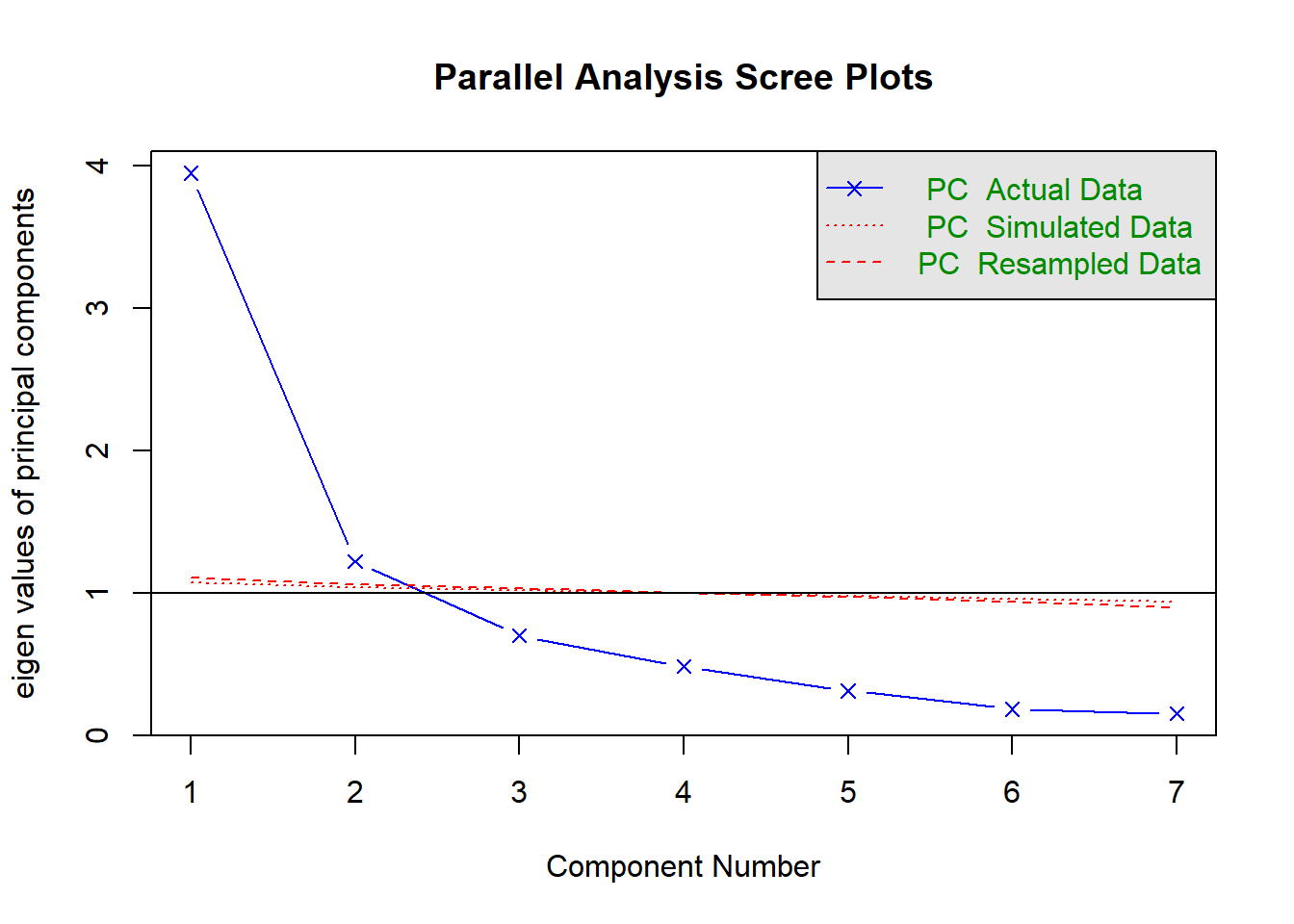
## Parallel analysis suggests that the number of factors = NA and the number of components = 2QUESTION 1. Examine the Scree plot. Does it support the hypothesis that only one factor underlies responses to Somatic Symptoms items? Why? Does your conclusion agree with the text output of the parallel analysis function?
Step 3. Interpreting parameters of a Graded Response Model
For IRT analyses, you will need package ltm (stands for “latent trait modelling”) installed on your computer. Select Tools / Install packages… from the RStudio menu, type in ltm and click Install. Make sure you load the installed package into the working memory before starting the below analyses.
To fit a Graded Response Model (GRM), use grm() function on somatic object containing item responses:
##
## Call:
## grm(data = somatic)
##
## Coefficients:
##          Extrmt1  Extrmt2  Extrmt3  Dscrmn
## SOMAT_1   -1.707    1.281    2.889   2.350
## SOMAT_2   -0.447    0.791    1.944   2.856
## SOMAT_3   -0.375    0.793    1.965   3.743
## SOMAT_4    0.270    1.231    2.332   3.223
## SOMAT_5    1.014    3.252    5.742   1.092
## SOMAT_6    1.328    2.895    5.392   1.234
## SOMAT_7    0.681    2.754    5.176   0.808
##
## Log.Lik: -15376.89
Examine the basic output above. Take note of the Log.Lik (log likelihood) at the end of the output. Log likelihood can only be interpreted in relative terms (compared to a log likelihood of another model), so you will have to wait for results from another model before using it.
Examine the Extremity and Discrimination parameters. Extremity parameters are really extensions of the difficulty parameters in binary IRT models, but instead of describing the threshold between two possible answers in binary items (e.g. ‘YES’ or ‘NO’), they contrast response category 1 with those above it, then category 2 with those above 2, etc. There are k-1 extremity parameters for an item with k response categories. In our 4-category items, Extrmt1 refers to the latent trait score z at which the probability of selecting any category >1 (2 or 3 or 4) equals 0.5. Below this point, selecting category 1 is more likely than selecting 2, 3 or 4; and above this point selecting categories 2, 3 or 4 is more likely. Extrmt2 refers to the latent trait score z at which the probability of selecting any categories >2 (3 or 4) equals 0.5. And Extrmt3 refers to the latent trait score z at which the probability of selecting any categories >3 (just 4) equals 0.5. The GRM assumes that the thresholds are ordered - that is, switching from one response category to the next happens at higher latent trait score values. That is why the GRM is a suitable model for Likert-type responses, which are supposedly ordered categories.
Discrimination refers to the steepness (slope) of the response characteristic curves at the extremity points. In GRM, this parameter is assumed identical for all categories, so the category curves have the same steepness.
This will be easier to understand by looking at Operation Characteristic Curves (OCC). These can be obtained easily by calling plot() function. If the default setting items=NULL is used, then OCCs will be produced for all items and the user can move from one to the next by hitting the Return key. To obtain OCC for a particular item, specify the item number:
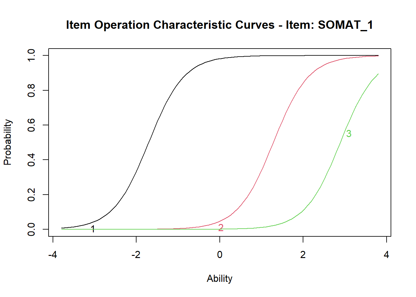
It can be seen that for item 1, Extrmt1= -1.707 is the trait score (the plot refers to it as “Ability” score) at which the OCC for category 1 crosses Probability 0.5; Extrmt2= 1.281 corresponds to the trait score at which OCC 2 crosses P=0.5, and Extrmt3= 2.889 corresponds to the trait score at which OCC 3 crosses P=0.5.
Plot and examine OCCs for all items.
QUESTION 2. Examine the OCC plots and the corresponding Extremity parameters. How are the extremities spaced out for different items? Do the extremity values vary widely? What are the most extreme values in this set? Examine the phrasing of the corresponding items – can you see why some categories are “easy” or “difficult” to select?
QUESTION 3. Examine the Discrimination parameters. What is the most and least discriminating item in this set? Examine the phrasing of the corresponding items – can you interpret the meaning of the construct we are measuring in relation to the most discriminating item (as we did for “marker” items in factor analysis)?
Now we are ready to look at Item Characteristic Curves (ICC) - the most useful plot in the practice of applying an IRT model. An ICC for each item will consist of as many curves as there are response categories, in our case 4. Each curve will represent the probability of selecting this particular response category, given the latent trait score. Let’s obtain the ICC for item SOMAT_3 by calling plot() function and specifying type="ICC":
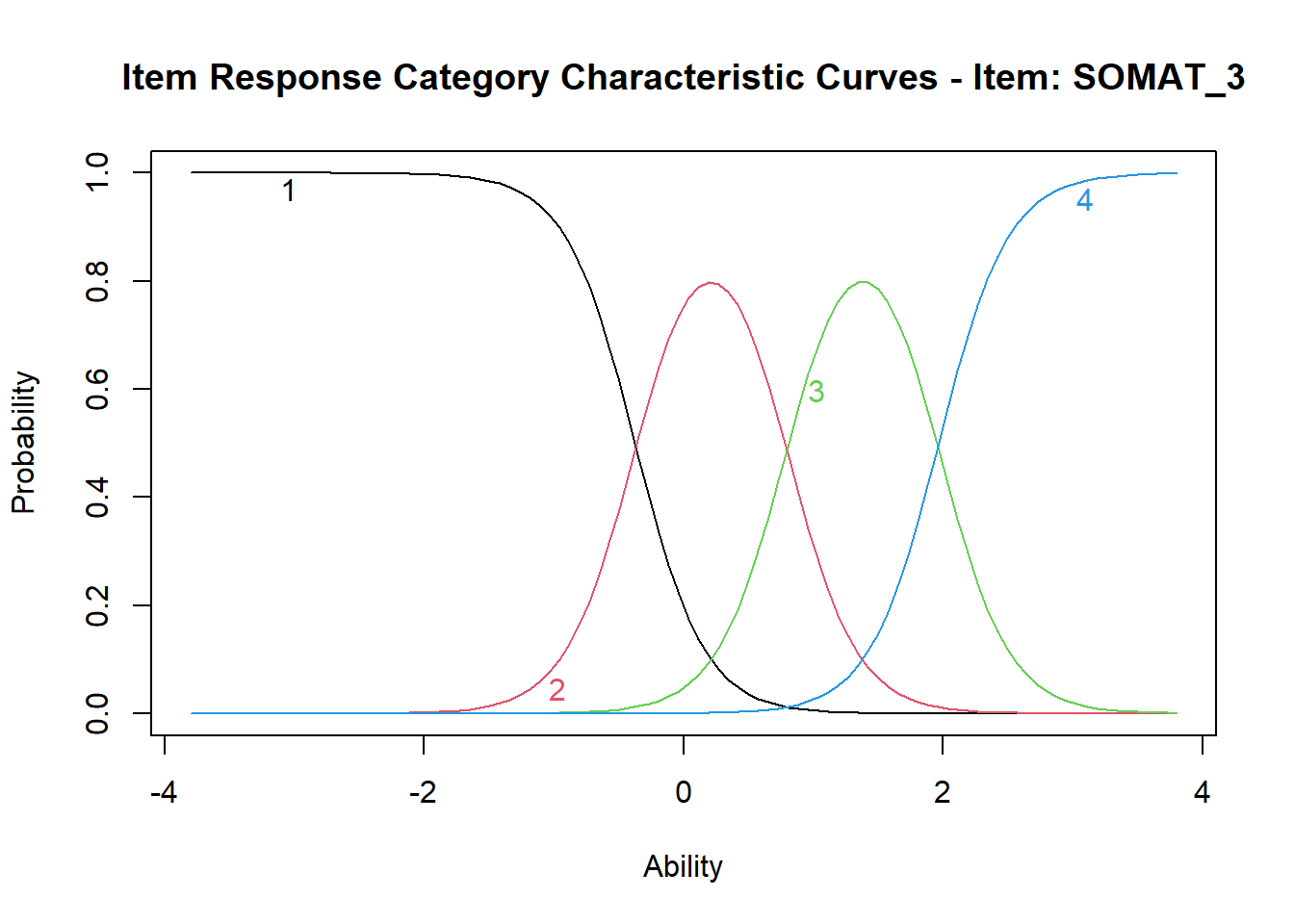
In this pretty plot, each response category from 1 to 4 has its own curve in its own colour. For item SOMAT_3 indicating distress, curve #1 (in black) represents the probability of selecting response “not at all”. You should be able to see that at the extremely low values of somatic symptoms (low distress), the probability of selecting this response approaches 1, and the probability goes down as the somatic symptoms score goes up (distress increases). Somewhere around Ability equal z=-0.5, the probability of selecting response #2 “no more than usual” plotted in pink becomes equal to the probability of selecting category #1 (the black and the pink lines cross), and then starts increasing as the somatic symptoms score goes up. The pink line #2 peaks somewhere around z=0.2 (which means that at this level of somatic symptoms, response #2 “no more than usual” is most likely), and then starts coming down. Then somewhere close to z=1, the pink line crosses the green line for response #3 “rather more than usual”, so that this response becomes more likely. Eventually, at about z=2 (high levels of distress), response #4 “much more than usual” (light blue line) becomes more likely and it reaches the probability close to 1 for extremely high z scores.
Plot and examine ICCs for all remaining items.Try to interpret the ICC for item SOMAT_1, which is the only item indicating health rather than distress. See how with the increasing somatic symptom score, the probability is decreasing for category #1 “better than usual” and increasing for category #4 “much worse than usual”.
Step 4. Testing alternative models and examining model fit
The standard GRM allows all items have different discrimination parameters, and we indeed saw that they varied between items. It would be interesting to see if these differences are significant - that is, if constraining the discrimination parameters equal resulted in a significantly worse model fit. We can check that by fitting a model where all discrimination parameters are constrained equal:
# discrimination parameters are constrained equal for all items
fit2 <- grm(somatic, constrained=TRUE)
fit2
##
## Call:
## grm(data = somatic, constrained = TRUE)
##
## Coefficients:
## Extrmt1 Extrmt2 Extrmt3 Dscrmn
## SOMAT_1 -1.798 1.406 3.122 1.789
## SOMAT_2 -0.423 1.346 2.814 1.789
## SOMAT_3 -0.360 1.340 2.929 1.789
## SOMAT_4 0.470 1.845 3.184 1.789
## SOMAT_5 0.830 2.367 4.173 1.789
## SOMAT_6 1.137 2.330 4.342 1.789
## SOMAT_7 0.480 1.663 2.963 1.789
##
## Log.Lik: -15668.06Examine the log likelihood (Log.Lik) for fit2, and note that it is different from the result for fit1.
You have fitted two IRT models to the Somatic Symptoms items. These models are nested - one is the special case of another (constrained model is a special case of the unconstrained model). The constrained model is more restrictive than the unconstrained model because it has fewer parameters (the same number of extremity parameters, but only 1 discrimination parameter in the constrained model against 7 in the unconstrained model, the difference of 6 parameters), and we can test which model fits better. Use the base R function anova() to compare the models - the more constrained one goes first:
##
##  Likelihood Ratio Table
##           AIC      BIC   log.Lik    LRT df p.value
## fit2 31380.12 31511.52 -15668.06
## fit1 30809.78 30977.02 -15376.89 582.34  6  <0.001
This function prints the Log.Lik values for the two models (you already saw them). It computes the likelihood ratio test (LRT) by multiplying each log likelihood by -2, and then subtracting the lower value from the higher value. The resulting value is distributed as chi-square, with degrees of freedom equal the difference in the number of parameters between the two models.
QUESTION 4. Examine the results of anova() function. LRT value is the likelihood ratio test result (the chi-square statistic). What are the degrees of freedom? Can you explain why the degrees of freedom are as they are? Is the difference between the two models significant? Which model would you retain and why?
Now, let’s see if the unconstrained GRM model (which we should prefer) fits the data well. For this, we will look at so-called two-way margins. They are obtained by taking two variables at a time, making a contingency table, and computing the observed and expected frequencies of bivariate responses under the GRM model (for instance, response #1 to item1 and #1 to item2; response #1 to item1 and #2 to item2 etc.). The Chi-square statistic is computed from each pairwise contingency table. A significant Chi-square statistic (greater than 3.8 for 1 degree of freedom) would indicate that the expected bivariate response frequencies are significantly different from the observed. This means that a pair of items have relationships beyond what is accounted for by the IRT model. In other words the local independence assumption of IRT is violated - the items are not independent controlling for the latent trait (dependence remains after the IRT model controls for the influences due to the latent trait). Comparing the observed and expected two-way margins is analogous to comparing the observed and expected correlations when judging the fit of a factor analysis model.
To compute these so called Chi-squared residuals, the package ltm has function margins().
##
## Call:
## grm(data = somatic)
##
## Fit on the Two-Way Margins
##
##         SOMAT_1 SOMAT_2 SOMAT_3 SOMAT_4 SOMAT_5 SOMAT_6 SOMAT_7
## SOMAT_1 -       449.93  501.91  373.66  148.71  152.32  149.56
## SOMAT_2 ***     -       328.58  253.63  154.07  153.28  145.72
## SOMAT_3 ***     ***     -       163.16  124.78  133.09  118.25
## SOMAT_4 ***     ***     ***     -       102.39   96.00   99.20
## SOMAT_5 ***     ***     ***     ***     -       879.46   80.40
## SOMAT_6 ***     ***     ***     ***     ***     -        82.40
## SOMAT_7 ***     ***     ***     ***     ***     ***     -
##
## '***' denotes pairs of items with lack-of-fit
QUESTION 5. Examine the Chi-squared residuals and find the largest one. Which pair of items does it pertain to? Can you interpret why this pair of items violates the local independence assumption?
The analysis of two-way margins confirms the results we obtained earlier from Parallel Analysis - that there is more than one factor underlying responses to the somatic items. At the very least, there is a second factor pertaining to a local dependency between two somatic items.
Step 5. Estimating trait scores for people
Now we can score people in this sample using function factor.scores() and Empirical Bayes method (EB). We will use the better-fitting 2PL model.
The estimated scores together with their standard errors will be stored for each respondent in a new object Scores. Check out what components are stored in this object by calling head(Scores). It appears that the estimated trait scores (z1) and their standard errors (se.z1) are stored in $score.dat part of the Scores object.
To make our further work with these values easier, let’s assign them to new variables in the GHQ data frame:
# Somatic Symptoms factor score
GHQ$somaticZ <- Scores$score.dat$z1
# Standard Error of the factor score
GHQ$somaticZse <- Scores$score.dat$se.z1
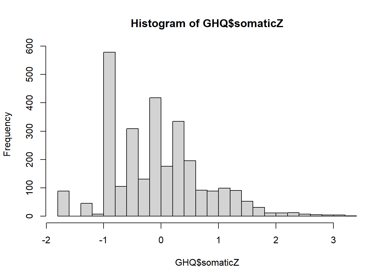
Now, you can plot the histogram of the estimated IRT scores, by calling
You can also examine relationships between the IRT estimated score and the simple sum score stored in the variable SUM_SOM. [Since there are no missing data, this variable can be computed by using function rowSums(somatic)].
You can plot the sum score against the IRT score.
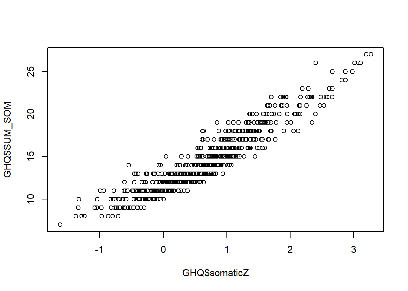
Note that the relationship between these scores is very strong, and almost linear. It is certainly more linear than the relationship in Exercise 12, which resembled a logistic curve. This suggests that the more response categories there are, the closer IRT models approximate linear models.
Step 6. Evaluating the Standard Errors of measurement
Now let’s plot the IRT estimated scores against their standard errors:
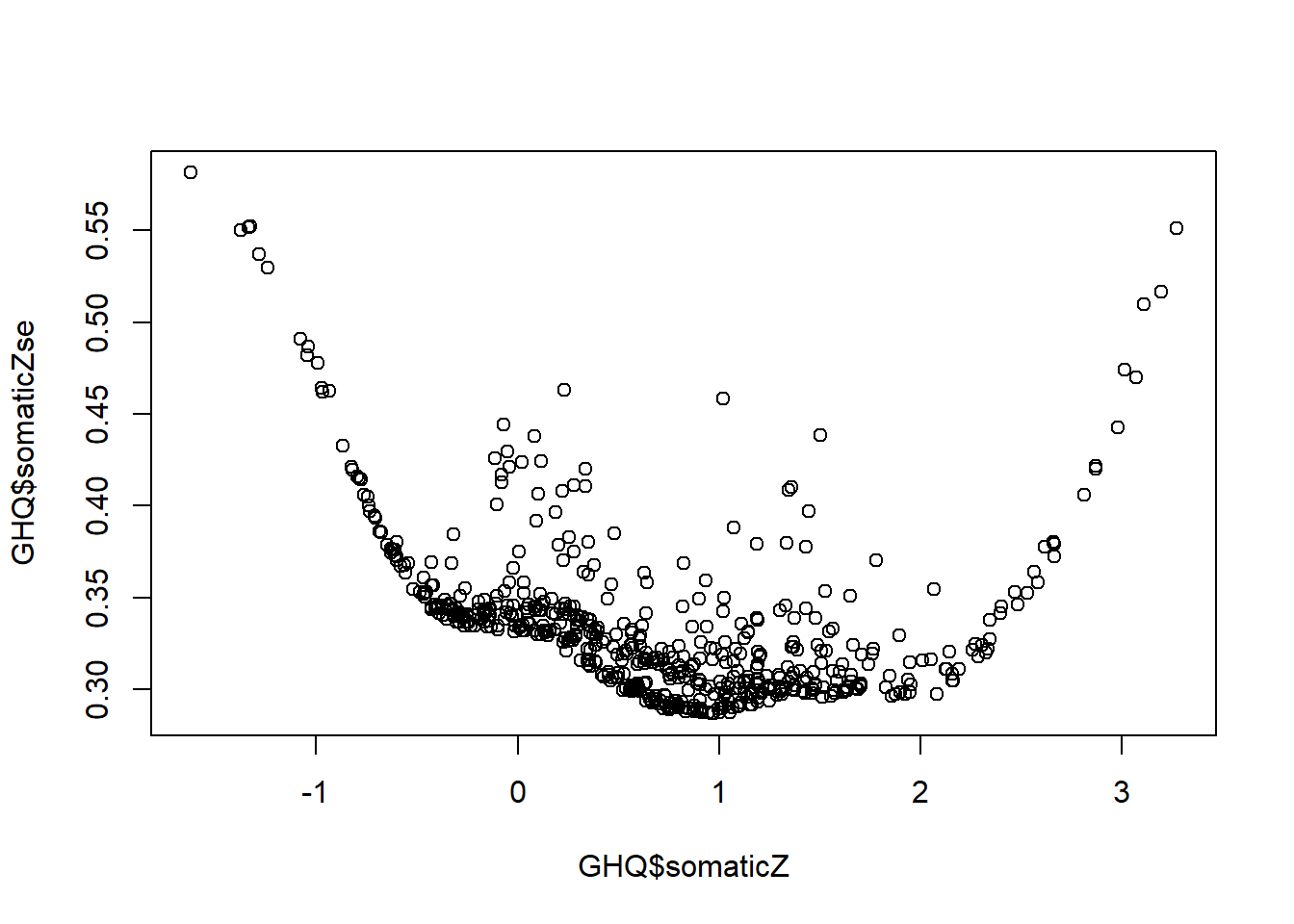
QUESTION 6. Examine the graph. What range of the somatic symptoms score is measured with most precision? What are the smallest and the largest Standard Errors on this graph, approximately?
[Hint. You can also get the exact values by calling min(GHQ$somaticZse) and max(GHQ$somaticZse).]
A very interesting feature of this graph is that some points are out of line with the majority (which form a relatively smooth curve). This means that Standard Errors can be different for people with the same latent trait score. Specifically, SEs can be larger for some people (note that the outliers are always above the trend, not below). The reason for it is that some individuals have aberrant response patterns - patterns not in line with the GRM model (for example, endorsing more ‘difficult’ response categories for some items while not endorsing ‘easier’ categories for other items). That makes estimating their score less certain.
Step 7. Saving your work
After you finished this exercise, you may want to save the new variables you created in the data frame GHQ. You may store the data in the R internal format (extension .RData), so next time you can use function load() to read it.
Before closing the project, do not forget to save your R script, giving it a meaningful name, for example “Fitting GRM model to GHQ”.
13.4 Solutions
Q1. According to the Scree plot of the observed data (in blue) the 1st factor accounts for a substantial amount of variance compared to the 2nd factor. There is a large drop from the 1st factor to the 2nd; however, the break from the steep to the shallow slope is not as clear as it could be, with the 2nd factor probably still being part of “the mountain” rather than part of “the rubble”. There are probably 2 factors underlying the data - one major explaining the most shared variance in the items, and one minor.
Parallel analysis confirms this conclusion, because the simulated data yields a line (in red) that crosses the observed scree between 2nd and 3rd factor, with 2nd factor significantly above the red line, and 3rd factor below it. It means that factors 1 and 2 should be retained, and factors 3, 4 and all subsequent factors should be discarded.
Q2. The extremity parameters vary widely between items. For SOMAT_2, SOMAT_3, and SOMAT_4, they are spaced more closely than for SOMAT_1 or SOMAT_5, SOMAT_6 and SOMAT_7.
The lowest threshold is between categories 1 and 2 of item SOMAT_1, with the lowest extremity value (Extrmt1=-1.707). SOMAT_1 is phrased “Have you recently: been feeling perfectly well and in good health?” (which is an item indicating health), and according to the GRM model, at the level of Somatic Symptoms z=–1.707 (which is well below the mean - remember, the trait score is scaled like z-score?), the probabilities of endorsing “1 = better than usual” and “2 = same as usual” are equal. People with Somatic Symptoms score lower than z=-1.707, will more likely say “1 = better than usual”, and with a score higher than z=-.707 (having more Somatic Symptoms) will more likely say “2 = same as usual”.
The highest threshold is between categories 3 and 4 of item SOMAT_5, with the lowest extremity value (Extrmt3=5.742). SOMAT_5 is phrased “Have you recently: been getting any pains in your head?” (which is an item indicating distress), and according to the GRM model, it requires an extremely high score of z=5.742 on Somatic Symptoms (more than 5 Standard Deviations above the mean) to switch from endorsing “3 = rather more than usual” to endorsing “4 = much more than usual”. It is easy to see why this item is more difficult to agree with than some other items indicating distress (which are all items except SOMATIC_1), as it refers to a pretty severe somatic symptom - head pains.
Q3. The most discriminating item in this set is SOMAT_3, phrased “Have you recently: been feeling run down and out of sorts?”. Apparently, this symptom is most sensitive to the change in overall Somatic Symptoms (a “marker” for this construct). The least discriminating item in this set is SOMAT_7, phrased “Have you recently: been having hot or cold spells?”. This symptom is less sensitive to the change in Somatic Symptoms (peripheral to the meaning of this construct).
Q4. The degrees of freedom for the likelihood ratio test is df=6. This is made up by the difference in the number of item parameters estimated. The unconstrained model estimated 7x3=21 extremity parameters and 7 discrimination parameters, 28 parameters in total. The constrained model estimated 7x3=21 extremity parameters and, only 1 discrimination parameter (one for all items), 22 parameters in total. The difference between the two models 28-22=6 parameters.
The chi-square value 582.34 on 6 degrees of freedom is highly significant, so the unconstrained GRM fits the data much better and we have to prefer it to the more parsimonious but worse fitting constrained model.
Q5. The largest Chi-squared residual is 879.46, pertaining to the pair SOMAT_5 (been getting any pains in your head?) and SOMAT_6 (been getting a feeling of tightness or pressure in your head?). It is pretty easy to see why this pair of items violates the local independence assumption. Both refer to one’s head - and experiencing “pain” is more likely in people who are also experience “pressure”, even after controlling for all other somatic symptoms. In other words, if we take people with exactly the same overall level of somatic symptoms (i.e. controlling for the overall trait level), those among them who experience “pain” will also more likely experience “pressure”. There is a residual dependency between these two symptoms.
Q6. The most precise measurement is observed in the range between about z=-0.5 and z=2.5. The smallest standard error was about 0.3 (exact value 0.287). The largest standard error was about 0.58 (exact value 0.581).