Exercise 12 Fitting 1PL and 2PL models to dichotomous questionnaire data.
| Data file | EPQ_N_demo.txt |
| R package | ltm |
12.1 Objectives
We already fitted a linear single-factor model to the Eysenck Personality Questionnaire (EPQ) Neuroticism scale in Exercise 8, using tetrachoric correlations of its dichotomous items. The objective of this exercise is to fit two basic Item Response Theory (IRT) models - 1-parameter logistic (1PL) and 2-parameter logistic (2PL) - to the actual dichotomous responses to EPQ Neuroticism items. After selecting the most appropriate response model, we will plot Item Characteristic Curves, and examine item difficulties and discrimination parameters. Finally, we will estimate people’s trait scores and their standard errors.
12.2 Worked Example - Fitting 1PL and 2PL models to EPQ Neuroticism items
To complete this exercise, you need to repeat the analysis from a worked example below, and answer some questions.
This exercise makes use of the data we considered in Exercises 6 and 8. These data come from a large cross-cultural study (Barrett, Petrides, Eysenck & Eysenck, 1998), with N = 1,381 participants who completed the Eysenck Personality Questionnaire (EPQ). The focus of our analysis here will be the Neuroticism/Anxiety (N) scale, measured by 23 items with only two response options - either “YES” or “NO”, for example:
N_3     Does your mood often go up and down?
N_7     Do you ever feel "just miserable" for no reason?
N_12    Do you often worry about things you should not have done or said?
etc.
You can find the full list of EPQ Neuroticism items in Exercise 6. Please note that all items indicate “Neuroticism” rather than “Emotional Stability” (i.e. there are no counter-indicative items).
Step 1. Opening and preparing the data
If you have already worked with this data set in Exercises 6 and 8, the simplest thing to do is to continue working within one of the projects created back then. In RStudio, select File / Open Project and navigate to the folder and the project you created. You should see the data frame EPQ appearing in your Environment tab, together with other objects you created and saved.
If you have not completed relevant exercises, or simply want to start from scratch, download the data file EPQ_N_demo.txt into a new folder and follow instructions from Exercise 6 on creating a project and importing the data.
The object EPQ should appear on the Environment tab. Click on it and the data will be displayed on a separate tab. As you can see, there are 26 variables in this data frame, beginning with participant id, age and sex (0 = female; 1 = male). These demographic variables are followed by 23 item responses, which are either 0 (for “NO”) or 1 (for “YES”). There are also a few missing responses, marked with NA.
Because the item responses are stored in columns 4 to 26 of the EPQ data frame, we will have to refer to them as EPQ[ ,4:26] in future analyses. More conveniently, we can create a new object containing only the item response data:
Step 2. Fit a 1-parameter logistic (1PL or Rasch) model
You will need package ltm (stands for “latent trait modelling”) installed on your computer. Select Tools / Install packages… from the RStudio menu, type in ltm and click Install. Make sure you load the installed package into the working memory:
To fit a 1-parameter logistic (1PL) model (which is mathematically equivalent to Rasch model), use rasch() function on N_data object with item responses:
Once the command has been executed, examine the model results by calling summary(fit1PL).
You should see some model fit statistics, and the estimated item parameters. Take note of the log likelihood (see Model Summary at the beginning of the output). Log likelihood can only be interpreted in relative terms (compared to a log likelihood of another model), so you will have to wait for results from another model before using it.
For item parameters printed in a more convenient format, call
##           Dffclt   Dscrmn
## N_3  -0.57725861 1.324813
## N_7  -0.18590831 1.324813
## N_12 -1.35483500 1.324813
## N_15  0.89517911 1.324813
## N_19 -0.32174146 1.324813
## N_23 -0.06547699 1.324813
## N_27  0.10182697 1.324813
## N_31  0.68572728 1.324813
## N_34 -0.41414515 1.324813
## N_38 -0.13645633 1.324813
## N_41  0.80993448 1.324813
## N_47 -0.34271380 1.324813
## N_54  0.78134781 1.324813
## N_58 -0.66528672 1.324813
## N_62  0.97477759 1.324813
## N_66 -0.34506389 1.324813
## N_68  0.25343459 1.324813
## N_72 -0.45539741 1.324813
## N_75  0.57519145 1.324813
## N_77  0.34614593 1.324813
## N_80 -0.45161535 1.324813
## N_84 -1.43292247 1.324813
## N_88 -2.03201824 1.324813
You should see the difficulty and discrimination parameters. Difficulty refers to the latent trait score at the point of inflection of the probability function (item characteristic curve or ICC); this is the point where the curve changes from concave to convex. In 1-parameter and 2-parameter logistic models, this point corresponds to the latent trait score where the probability of ‘YES’ response equals the probability of ‘NO’ response (both P=0.5). Discrimination refers to the steepness (slope) of the ICC at the point of inflection (at the item difficulty).
QUESTION 1. Examine the 1PL difficulty parameters. Do the difficulty parameters vary widely? What is the ‘easiest’ item in this set? What is the most ‘difficult’ item? Examine the phrasing of the corresponding items (refer to the item list in Appendix) – can you see why one item is easier to agree with than the other?
QUESTION 2. Examine the 1PL discrimination parameters. Why is the discrimination parameter the same for every one of 23 items?
Now plot item characteristic curves for this model using plot() function:
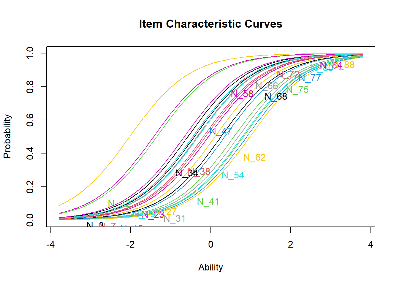
Examine the item characteristic curves (ICCs). First, you should notice that they run in “parallel” to each other, and do not cross. This is because the slopes are constrained to be equal in the 1PL model. Try to estimate the difficulty levels of the most extreme items on the left and on the right, just by looking at the approximate trait values where corresponding probabilities equal 0.5. Check if these values equal to the difficulty parameters printed in the output.
Step 3. Fit a 2-parameter logistic model
To fit a 2-parameter logistic (2PL) model, use ltm() function (stands for ‘latent trait model’) as follows:
The function uses a formula, described in the ltm package manual. The formula follows regression conventions used by base R and many packages – it specifies that items in the set N_data are ‘regressed on’ (~) one latent trait (z1). Note that z1 is not an arbitrary name; it is actually fixed in the package. At most, two latent traits can be fitted (z1 + z2). We are only fitting one trait and therefore we specify ~ z1.
When the command has been executed, see the results by calling summary(fit2PL).
You should see some model fit statistics, and then estimated item parameters – difficulties and discriminations. Take note of the log likelihood for this model. We will test how the 2PL model compares to the 1PL model later using this value.
For the item parameters printed in a convenient format, call
##           Dffclt    Dscrmn
## N_3  -0.51605652 1.6321883
## N_7  -0.17666140 1.4774008
## N_12 -1.22040224 1.5911491
## N_15  1.03197005 1.0570904
## N_19 -0.26737063 1.9740413
## N_23 -0.06402011 1.5006632
## N_27  0.09002533 1.5308778
## N_31  0.59894671 1.6672151
## N_34 -0.32318252 2.3270028
## N_38 -0.13268055 1.4266667
## N_41  0.75664387 1.4738613
## N_47 -0.52960514 0.7057917
## N_54  1.08776504 0.8186594
## N_58 -0.69064694 1.2397378
## N_62  1.05886259 1.1532931
## N_66 -0.42109219 0.9640119
## N_68  0.32362475 0.9217228
## N_72 -0.40104331 1.6932412
## N_75  0.48193055 1.8070986
## N_77  0.31094924 1.5627476
## N_80 -0.42017648 1.5126054
## N_84 -1.92770607 0.8595893
## N_88 -2.57944224 0.9375370
QUESTION 3. Examine the 2PL difficulty parameters. What is the ‘easiest’ item in this set? What is the most ‘difficult’ item? Are these the same as in the 1PL model? Examine the phrasing of the corresponding items – can you see why one item is much easier to agree with than the other?
QUESTION 4. Examine the 2PL discrimination parameters. What is the most and least discriminating item in this set? Examine the phrasing of the corresponding items – can you interpret the meaning of the construct we are measuring in relation to the most discriminating item (as we did for “marker” items in factor analysis)?
Now plot item characteristic curves for this model:
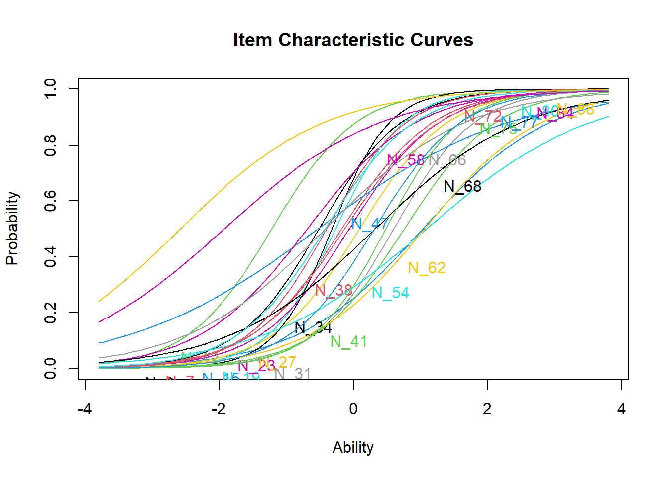
QUESTION 5. Examine the item characteristic curves. Now the curves should cross. Can you identify the most and the least discriminating items from this plot?
Step 4. Compare 1PL and 2PL models
You have fitted two IRT models to the Neuroticism items. These models are nested - one is the special case of another (1PL model is a special case of 2PL with all discrimination parameters constrained equal). The 1PL (Rasch) model is more restrictive than the 2PL model because it has fewer parameters (23 difficulty parameters and only 1 discrimination parameter, against 23 difficulties + 23 discrimination parameters in the 2PL model), and we can test which model fits better. Use the base R function anova() to compare the models:
##
##  Likelihood Ratio Table
##             AIC      BIC   log.Lik    LRT df p.value
## fit1PL 34774.05 34899.59 -17363.03
## fit2PL 34471.99 34712.60 -17189.99 346.06 22  <0.001
This function prints the log likelihood values for the two models (you already saw them). It computes the likelihood ratio test (LRT) by multiplying each log likelihood by -2, and then subtracting the lower value from the higher value. The resulting value is distributed as chi-square, with degrees of freedom equal the difference in the number of parameters between the two models.
QUESTION 6. Examine the results of anova() function. LRT value is the likelihood ratio test result (the chi-square statistic). What are the degrees of freedom? Can you explain why the degrees of freedom as they are? Is the difference between the two models significant? Which model would you retain and why?
Step 5. Estimate Neuroticism trait scores for people
Now we can score people in this sample using function factor.scores() and Empirical Bayes method (EB). We will use the better-fitting 2PL model.
The estimated scores together with their standard errors will be stored for each respondent in a new object Scores. Check out what components are stored in this object by calling head(Scores). It appears that the estimated trait scores (z1) and their standard errors (se.z1) are stored in $score.dat part of the Scores object.
To make our further work with these values easier, let’s assign them to new variables in the EPQ data frame:
# the Neuroticism factor score
EPQ$Zscore <- Scores$score.dat$z1
# Standard Error of the factor score
EPQ$Zse <- Scores$score.dat$se.z1
Now, you can plot the histogram of the estimated IRT scores, by calling hist(EPQ$Zscore).
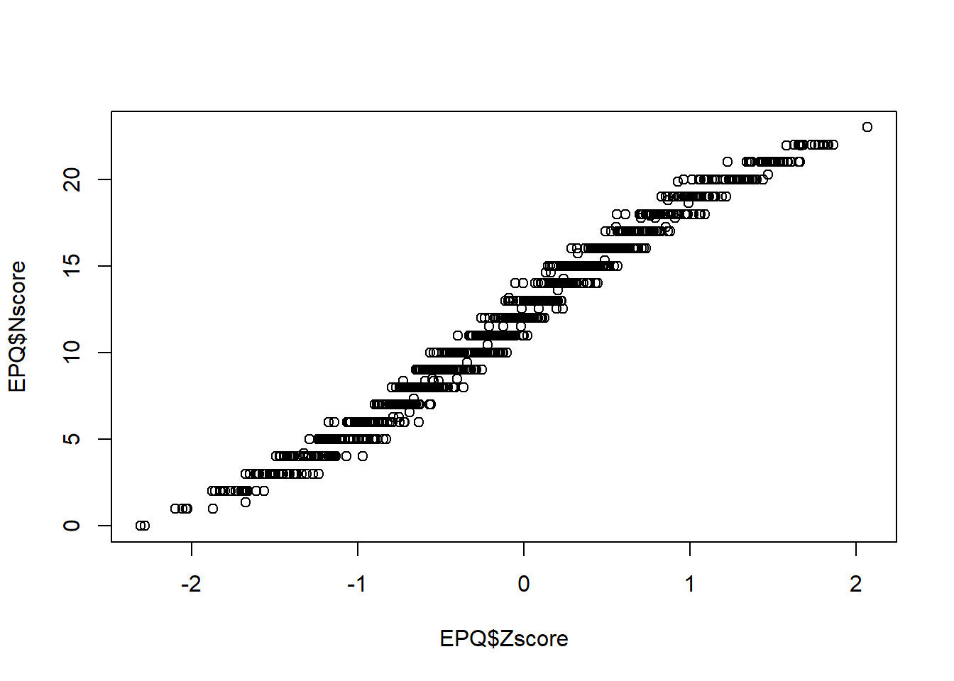
You can also examine relationships between the IRT estimated scores and simple sum scores. This is how we computed the sum scores previously in Exercise 6:
Then plot the sum score against the IRT score. Note that the relationship between these scores is very strong but not linear. Rather, it resembles a logistic curve.
Step 6. Evaluate the Standard Errors of measurement
Now let’s plot the IRT estimated scores against their standard errors:
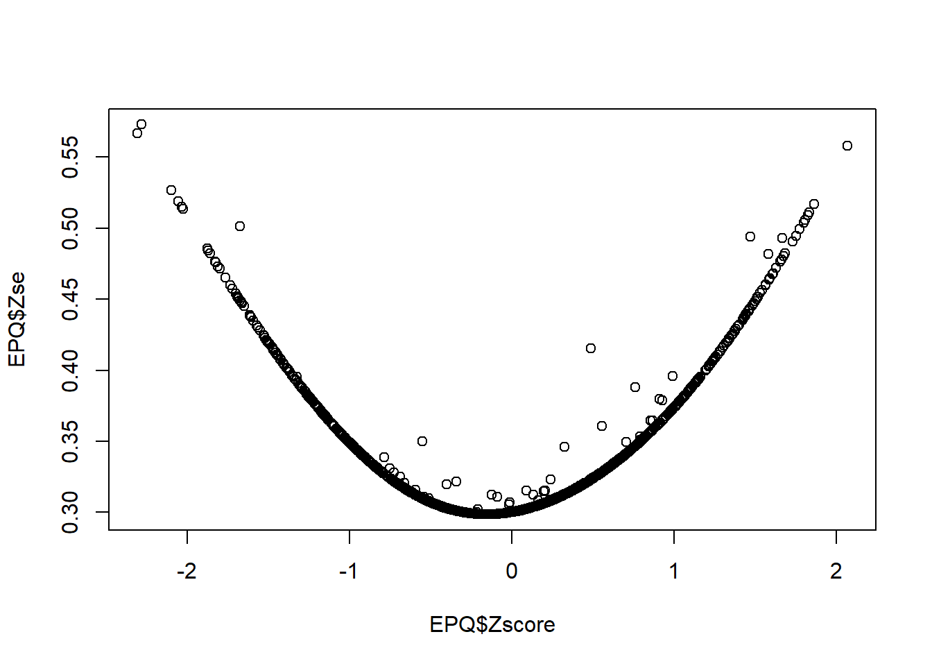
QUESTION 7. Examine the graph. What range of the Neuroticism trait score is measured with most precision? What are the smallest and the largest Standard Errors on this graph, approximately?
[Hint. You can also get the exact values by calling min(EPQ$Zse) and max(EPQ$Zse).]
A very interesting feature of this graph is that a few points are out of line with the majority (which form a very smooth curve). This means that SEs can be different for people with the same latent trait score. Specifically, SEs can be larger for some people (note that the outliers are always above the trend, not below). The reason for it is that some individuals had missing responses, and because fewer items provided information for their score estimation, their SEs were larger than for individuals with complete response sets.
Step 7. Saving your work
After you finished this exercise, you may close the project. Do not forget to save your R script, giving it a meaningful name, for example “IRT analysis of EPQ_N”.
Please also make sure that you save your entire ‘workspace’, which includes the data frame and all the new objects you created. This will be useful for your revision.
12.3 Solutions
Q1. The difficulty parameters of Neuroticism items vary widely. The ‘easiest’ item to endorse is N_88, with the lowest difficulty value (-2.03). N_88 is phrased “Are you touchy about some things?”, and according to the 1PL model, at very low neuroticism level z=–2.03 (remember, the trait score is scaled like z-score), the probability of agreeing with this item is already 0.5. The most ‘difficult’ item to endorse in this set is N_62, with the highest difficulty value (0.97). N_62 is phrased “Do you often feel life is very dull?”, and according to this model, one needs to have neuroticism level of at least 0.97 to endorse this item with probability 0.5. The phrasing of this item is indeed more extreme than that of item N_88, and it is therefore more ‘difficult’ to endorse.
Q2. Only one discrimination parameter is printed for this set because the 1PL (Rasch) model assumes that all items have equal discriminations. Therefore the model constrains all discriminations to be equal.
Q3. The ‘easiest’ item to endorse in this set is still item N_88, which now has the difficulty value -2.58. The most ‘difficult’ item to endorse in this set is now item N_54, with the difficulty value (1.09). The most difficult item from the 1PL model, N_62, has a similarly high difficulty (1.06). N_54 is phrased “Do you suffer from sleeplessness?”, and according to this model, one needs to have neuroticism level of at least 1.09 to endorse this item with probability 0.5.
Q4. The most discriminating item in this set is N_34 (Dscrmn.=2.33). This item reads “Are you a worrier?”, which seems to be right at the heart of the Neuroticism construct. This is the item which would have the highest factor loading in factor analysis of these data. The least discriminating item is N_47 (Dscrmn.=0.71), reading “Do you worry about your health?”. According to this model, the item is more marginal to the general Neuroticism construct (perhaps it tackles a context-specific behaviour).
Q5. The most and the least discriminating items can be easily seen on the plot. The most discriminating item N_34 has the steepest slope, and the least discriminating item N_47 has the shallowest slope.
Q6. The degrees of freedom = 22. This is made up by the difference in the number of item parameters estimated. The Rasch model estimated 23 difficulty parameters, and only 1 discrimination parameter (one for all items). The 2PL model estimated 23 difficulty parameters, and 23 discrimination parameters. The difference between the two models = 22 parameters.
The chi-square value 346.06 on 22 degrees of freedom is highly significant, so the 2PL model fits the data much better and we have to prefer it to the more parsimonious but worse fitting 1PL model.
Q7. Most precise measurement is achieved in the range between about z=-0.2 and z=0. The smallest standard error was about 0.3 (exact value 0.299). The largest standard error was about 0.57 (exact value 0.573).