4.4 Temporal Confounding

Let’s first consider a simple linear regression model,

$$y_t = \beta x_t + \varepsilon_t$$

where $t=0,\dots,n-1$ and $\varepsilon_t$ is a Gaussian process with mean $0$ and autocovariance $\sigma^2\rho(u)$. For now, without loss of generality, let’s assume that $\mathbb{E}[y_t]=\mathbb{E}[x_t]=0$ and that $\text{Var}(x_t)=1$. The least squares estimate for $\beta$ is

$$\hat{\beta} = \frac{1}{n}\sum_{t=0}^{n-1} y_t x_t.$$ Strictly speaking, $\beta$ quantifies the strength of the association between $x_t$ and $y_t$ at 0-lag. If $t$ represents the time unit of a “day”, then $\beta$ is the 0-day lag association.

Based on what we learned in the chapter on frequency and time scale analysis, we can decompose $x_t$ into its Fourier components,

$$x_t = \frac{1}{n}\sum_{p=0}^{n-1}z_x(p)\exp(2\pi i pt/n)$$ (assuming that $n$ is even for now), where $z_x(p)$ is the complex Fourier coefficient associated with the frequency $p$ and the series $x_t$, i.e.

$$z_x(p)=\sum_{t=0}^{n-1}x_t\exp(-2\pi i pt/n).$$

Plugging into the formula for the least squares estimate gives us an estimate of $\beta$ as

$$\begin{eqnarray*} \hat{\beta} & = & \frac{1}{n}\sum_{t=0}^{n-1} y_t x_t\\ & = & \frac{1}{n} \sum_{t=0}^{n-1} y_t \left[ \frac{1}{n}\sum_{p=0}^{n-1}z_x(p)\exp(2\pi i pt/n) \right]\\ & = & \frac{1}{n^2}\sum_{t=0}^{n-1}\sum_{p=0}^{n-1} z_x(p)y_t\exp(2\pi i pt/n)\\ & = & \frac{1}{n^2}\sum_{p=0}^{n-1} \left[ z_x(p) \sum_{t=0}^{n-1} y_t\exp(2\pi i tp/n) \right]\\ & = & \frac{1}{n^2}\sum_{p=0}^{n-1} z_x(p)\bar{z}_y(p) \end{eqnarray*}$$ where $\bar{z}_y(p)$ is the complex conjugate of the Fourier coefficient associated with the series $y_t$ at frequency $p$.

The derivation above shows that the least squares estimate of the coefficient $\beta$ can be written as a sum of the products of the Fourier coefficients between the $y_t$ and $x_t$ series over all of the frequencies. While it’s not advisable to compute $\hat{\beta}$ in this manner as it would require two separate FFTs (one for $y_t$ and one for $x_t$), it does show the dependence on $\hat{\beta}$ on all of the time scales of variation in both $y_t$ and $x_t$.

One of the primary advantages of doing regression of time series data is that we can decided for ourselves what time scales of variation we are in fact interested in. It is not necessary for us to focus our attention on all of the time scales of variation in the (as the naive least squares estimate would have us do) if some of the time scales to not have a meaningful interpretation. For example, if we are primarily interested in long-term trends in $x_t$ and $y_t$, then we do not need to focus on the high-frequency components. Similarly, if we are interested in short-term fluctuations between $x_t$ and $y_t$, then we can discard the low-frequency components of $\hat{\beta}$.

We can think of the $\hat{\beta}$ as being a mixture of associations at different time scales, and we may focus our attention on only those associations/time scales that are of interest to us. If we let

$$\hat{\beta}_p = \frac{z_x(p)}{n}\frac{\bar{z}_y(p)}{n}$$

then we can write the least squares estimate as

$$\hat{\beta}_{LS} = \sum_{p=0}^{n-1} \hat{\beta}_p.$$

The point of showing this is that we rarely are focused on the association between $x_t$ and $y_t$ at all time scales at the same time. In any given analysis, we may be focused on short-term associations (e.g. “acute” effects) or we may be focused on long-term associations. But it’s rarer to want to mix all of those associations together. However, that’s exactly what the least squares estimate does.

4.4.1 Bias from Omitted Temporal Confounders

A well-known result in the theory of least squares estimators is one due to omitted variable bias. Suppose the true model for $y_t$ is

$$y_t = \beta x_t + \gamma w_t + \varepsilon_t$$

where $z_t$ is some other time series with mean $0$ and variance $1$. If we include $x_t$ but omit $z_t$ from our modeling and simply estimate $\beta$ via least squares, we will get

$$\begin{eqnarray*} \hat{\beta}_{LS} & = & \frac{1}{n} \sum_{t=0}^{n-1} y_t x_t\\ & = & \frac{1}{n} \sum_{t=0}^{n-1} (\beta x_t + \gamma w_t + \varepsilon_t) x_t\\ & = & \beta\widehat{\text{Var}}(x_t) + \gamma\frac{1}{n}\sum_{t=0}^{n-1} w_t x_t + \frac{1}{n}\sum_{t=0}^{n-1}\varepsilon_t x_t\\ & \approx & \beta + \gamma\frac{1}{n}\sum_{t=0}^{n-1} w_t x_t\\ \end{eqnarray*}$$

So the bias in the least squares estimate of $\beta$ is equal to $\gamma\frac{1}{n}\sum_{t=0}^{n-1} w_t x_t$. However, notice that the quantity $\frac{1}{n}\sum_{t=0}^{n-1} w_t x_t$ is essentially the least squares estimate of the coefficient in the simple linear regression model relating $w_t$ to $x_t$, i.e. it is the emprical covariance between $w_t$ and $x_t$. Of course, this implies that if the covariance between $w_t$ and $x_t$ is zero, then there is no bias in $\hat{\beta}_{LS}$ and there is no danger in omitting $w_t$ from the model for $y_t$. But we can also write the bias as a sum of Fourier coefficients,

$$\text{Bias}(\hat{\beta}_{LS}) = \gamma \frac{1}{n^2} \sum_{p=0}^{n-1} z_w(p)\bar{z}_x(p)$$

From this representation, we can see that one way to eliminate (or at least minimize) the bias from omitting the variable $w_t$ is to focus on time scales $p$ where either $z_w(p) \approx 0$. As long as there is no time scale where the Fourier coefficients for both $x_t$ and $w_t$ are large, the bias should be close to zero. Also, it’s worth noting that if $\gamma = 0$ there is no bias, but for now we will assume that $\gamma\ne 0$.

4.4.2 Example: Confounding by Smoothly Varying Factors

For example, suppose we are looking at temperature and mortality and we are concerned about possible confounding by economic development. Urban economic development is correlated with the “urban heat island” effect as more roads and building can cause increased temperatures in urban environments. Furthermore, economic development can be related to mortality in a variety of ways.

One assumption we might be willing to make is that economic development largely occurs over broad time scales, on the order of months to years or even decades. As such, most of the variation in any variable that tracked economic development would be concentrated in the low frequencies. Therefore, if we focus our interest on variation temperature and mortality in the higher frequency ranges, where we might assume that the Fourier coefficients for economic development are close to $0$ (but the coefficients for temperature and mortality are non-zero), then we may be less concerned about confounding from that particular factor.

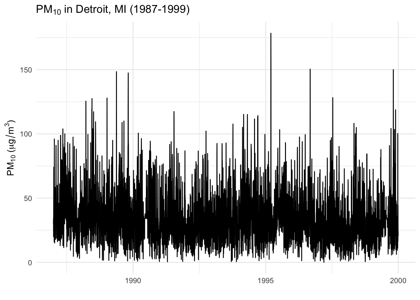
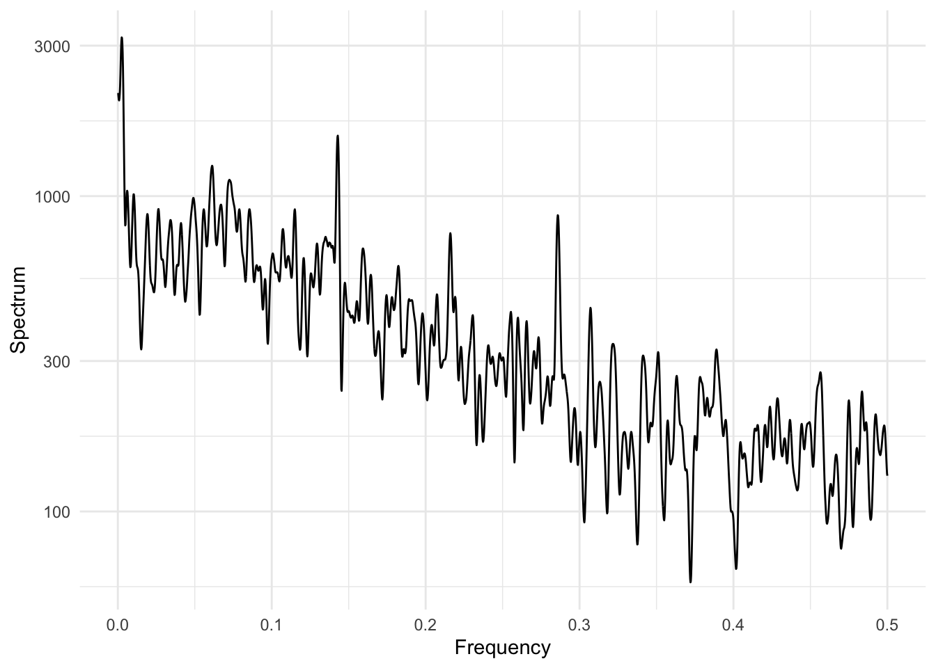
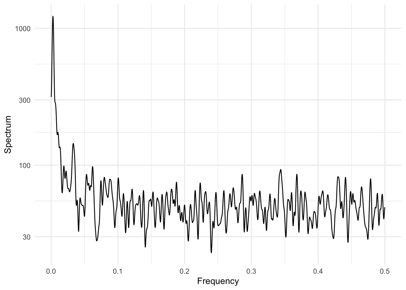
As another example, suppose we are interested in studying air pollution and mortality and are worried about possible confounding by seasonally varying factors. Seasonal factors have a strong variation at 1 cycle per year ($\approx 365$ days) and so we might want to focus our interest in looking at variation in air pollution and mortality either at shorter time scales or at longer time scales.