5.9 Exponential Smoothing

NOTE: I don’t know where this section is supposed to go.

Suppose we have an ongoing time series $y_1, y_2, \dots$ and we want to make a prediction about $y_{t+1}$ given the past $y_t, y_{t-1}, y_{t-2}, \dots$. The exponential smoothing approach takes a value $\lambda\in (0, 1)$ and produces

$$\hat{y}_{t+1} = (1-\lambda)\sum_{j=0}^\infty \lambda^j y_{t-j}$$ This forecasted value weights the previous values with the weights decreasing geometricallly as the values go further back in time.

Although the sum is infinite, we can see readily that

$$\begin{eqnarray*} \hat{y}_{t+1} & = & (1-\lambda) \left[ y_t + \lambda y_{t-1} + \lambda^2 y_{t-2} + \cdots \right]\\ & = & (1-\lambda)y_t + (1-\lambda)\sum_{j=1}^\infty\lambda^jy_{t-j}\\ & = & (1-\lambda)y_t + \lambda(1-\lambda)\sum_{j=0}^\infty\lambda^jy_{t-1-j}\\ & = & (1-\lambda)y_t + \lambda \hat{y}_t \end{eqnarray*}$$

So from the infinite sum we can derive a rather simple recursion. Furthermore, this recursion can be re-written as

$$\begin{eqnarray*} \hat{y}_{t+1} & = & (1-\lambda)y_t + \lambda \hat{y}_t - \hat{y}_t + \hat{y}_t\\ & = & (1-\lambda)y_t -\hat{y}_t (1-\lambda) + \hat{y}_t\\ & = & \hat{y}_t + (1-\lambda)(y_t-\hat{y}_t) \end{eqnarray*}$$

Here, the prediction for time $t+1$ is written as the predicted value for time $t$ plus the deviation of the observed $y_t$ and the predicted $\hat{y}_t$. In this way, the exponential smoother is incorporating new data while giving some weight to the predicted value. It is clear that if $\lambda=1$, we stick with our predicted values and if $\lambda=0$ we go with the new observed value. For values between $0$ and $1$ we average between the two.

One way to choose $\lambda$ is to choose it based on how far back you want values to influence the current prediction. For example, for a “90-day” exponential smooth, we might choose $\lambda$ such that $\lambda^j < \varepsilon$ for $j > 90$ and $\varepsilon$ very small. For example, for $\varepsilon = 0.00001$, we would want $\lambda < 0.00001^{1/90} \approx 0.88$.

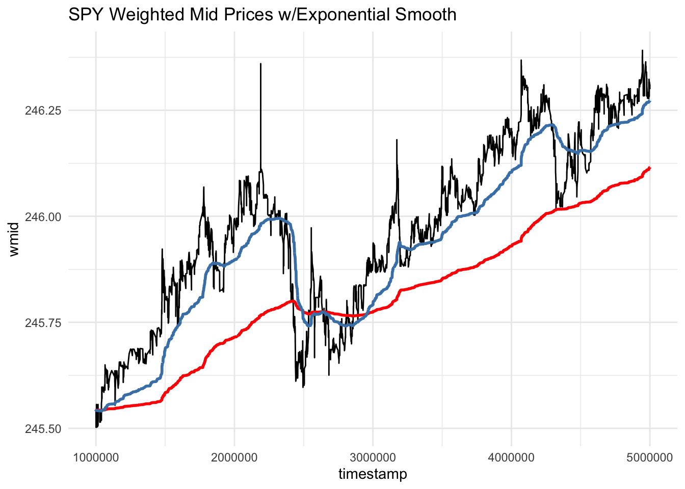
A common stock chart for “technical analysis” is to plot a stock’s observed prices along with various exponential smooths with differing weights. If the current observed price is above one of the smoothed averages it might be considered “over-bought”, while if the observed price is below one of the averages it might be considered “over-sold”. Be forewarned that this is not financial advice!

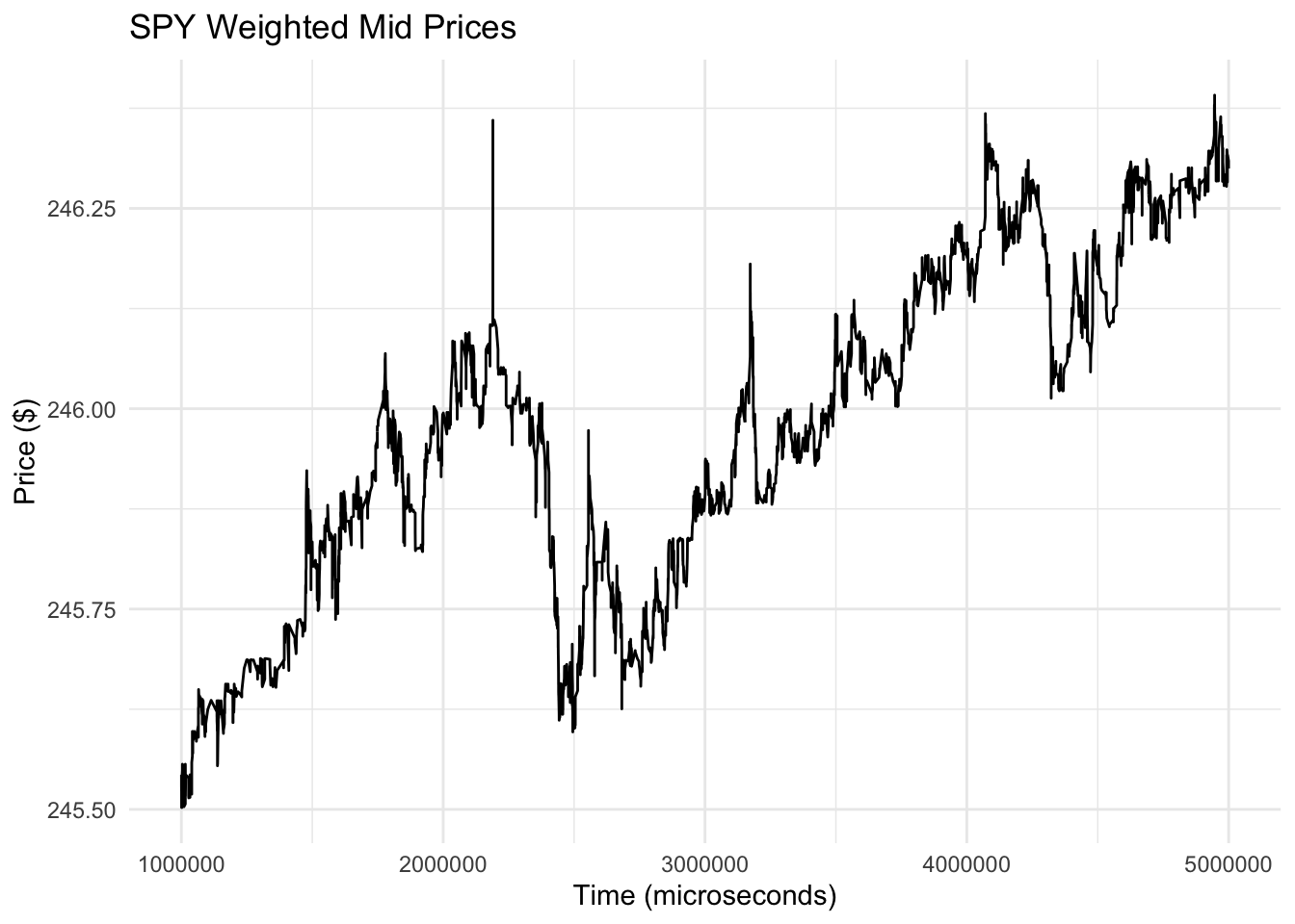
Here is a plot of the weighted mid price for the SPY exchange traded fund for a few seconds of trading.

Here is the same plot with two exponential smooths, one with $\lambda=0.995$ and one with $\lambda=0.999$.