2.7 Stationarity
Stationarity of a series \(X_1,X_t,\dots\) is a critical property that allows us to apply many of the standard tools of time series analysis.
A time series is strictly stationary if for any subset of size \(n\) and any integer \(\tau\), \((Y_{t_1}, Y_{t_2},\dots,Y_{t_n})\) has the same joint distribution as \((Y_{t_1+\tau}, Y_{t_2+\tau},\dots,Y_{t_n+\tau})\).
In other words, from a distributional standpoint, a stationary time series is invariant to shifts
Because the definition holds for all \(n\), including \(n=1\), we have that the mean and variance of the \(Y_t\) is constant for all \(t\).
Sometimes strict stationarity is too difficult to require, so we usually use a weaker concept.
A time series is second-order stationary if the mean is constant and the covariance between any two values only depends on the time difference between those two values (and not on the value of \(t\) itself).
\(\mathbb{E}[Y_t] = \mu\).
\(\text{Cov}(Y_t, Y_{t+\tau}) = \gamma(\tau)\), a function of \(\tau\) only.
The function \(\gamma()\) is known as the auto-covariance function.
For the most part here, we will assume that time series are second-order stationary and not concern ourselves with the higher moments of the joint distribution of the data.
The basic idea of stationarity is that the distribution of the data does not depend on \(t\), so knowledge of \(t\) itself does not tell you anything about the distribution. This allows us to consider the time series as “stable” over time so that while there may be random deviations from time to time, there will not be major changes in the distribution over time.
Stationarity can be thought of in the following way: Imagine you’re “looking” at your time series at the moment. Then we fast foward the clock 6 months and you’re looking at the time series as it would appear 6 months later. Does it look fundamentally different? Sure, there would be random variations in the value, but if I hadn’t told you it was 6 months later, would you be able to tell that the time had shifted? If the answer is “no”, then the time series is stationary.
Consider another example: Imagine you’re following the time series of temperature in your city and at the moment it’s winter. Now if I were to fast forward 6 months, things would look very different. It would be summer and the temperature would be a lot warmer. It would be obvious that we had traveled in time. This is an example of a time series that is not stationary because the distribution of the data depends on the the time itself.
Now consider the following scenario: Imagine you’re looking at the hourly temperature in your city over time for the current week. Then I shift you one week into the future. Would the time series of hourly temperatures look very different from the week before? Probably not, because the time shift is relatively small. This suggests that the time scale of variation that we are considering plays a role in whether we think of a time series as stationary. It may not be realistic to think of a time series as stationary over 6-month time shifts, but it may be more reasonable to think of it as stationary over 1-week time shifts.
But the definition of stationarity says the property should hold for all time shifts. So what is a practical thing we can do?
Consider the plot below, which shows daily average temperature for the city of Baltimore, MD in 2005.
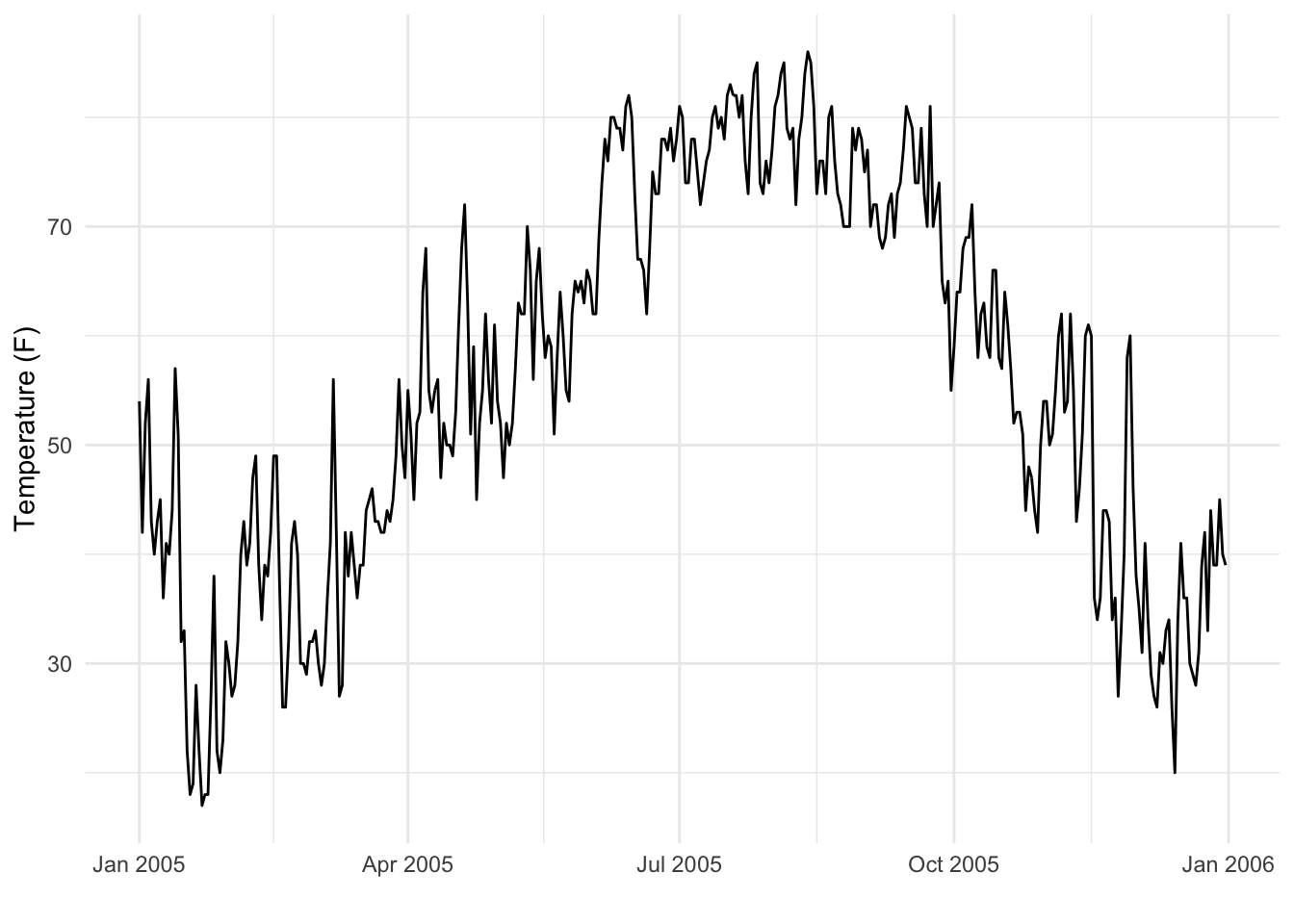
As one might expect, there is a strong seasonal pattern with temperatures lower in the winter months and higher in the summer months. Clearly, the series is non-stationary because knowing that it is July gives you substantial information about the distribution of the temperature data.
The plot below shows the residuals after fitting a linear model with a constant monthly effect.
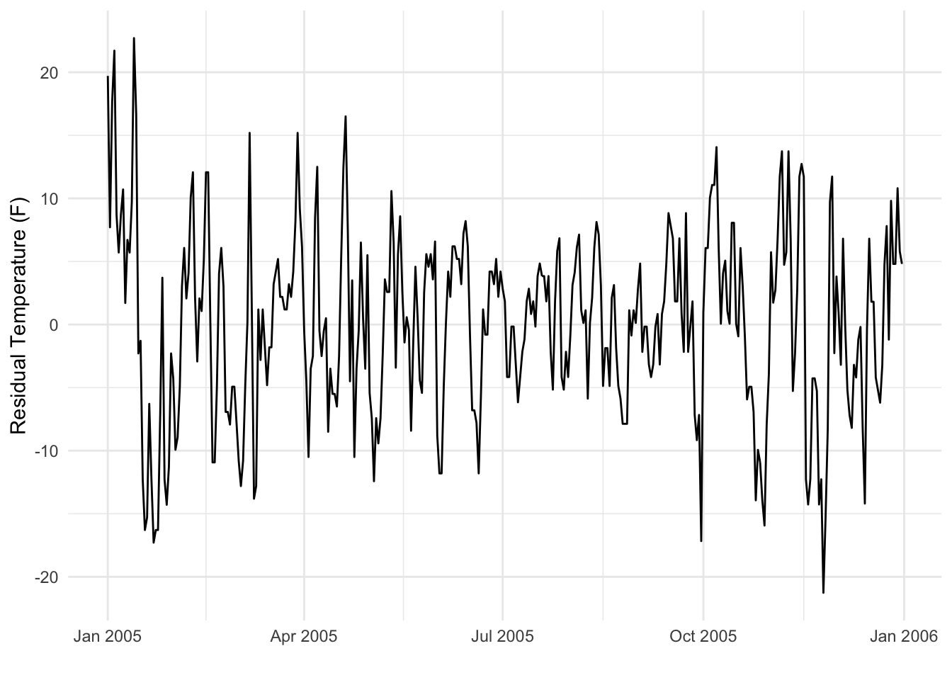
This plot does show some pattern, primarily in its variability over time, but the overall mean is zero, as it should be after fitting a linear model. It might be reasonable to argue that this series looks “more stationary” with the monthyl trend removed than the previous one. However, the variance does appear to be larger in the winter months than the summer months.
The bottom line here is that the temperature series had a strong fixed effect, which was the seasonal pattern. After removing that fixed effect we could make a somewhat better argument that the residual variation was stationary. In traditional regression settings we might assume that the residual variation is independent and identically distributed (iid), but in the time series context, there might be some residual autocorrelation remaining, even if the series is stationary.