6.3 Example: A Local Level Model

We can use as a simple example the local level model specified with the following observation and state equations:

\[\begin{eqnarray*} y_t & = & A x_t + \varepsilon_t\\ x_t & = & \theta x_{t-1} + \eta_t \end{eqnarray*}\]

where \(\varepsilon\sim\mathcal{N}(0,\sigma^2)\) and \(\eta_t\sim\mathcal{N}(0,\tau^2)\). In this model, we have \(\boldsymbol{\beta} = (A, \theta,\sigma, \tau)\). We also need initial values for \(x_0^0\) and \(P_0^0\), which we can either assume as known or include in the vector of unknown parameters.

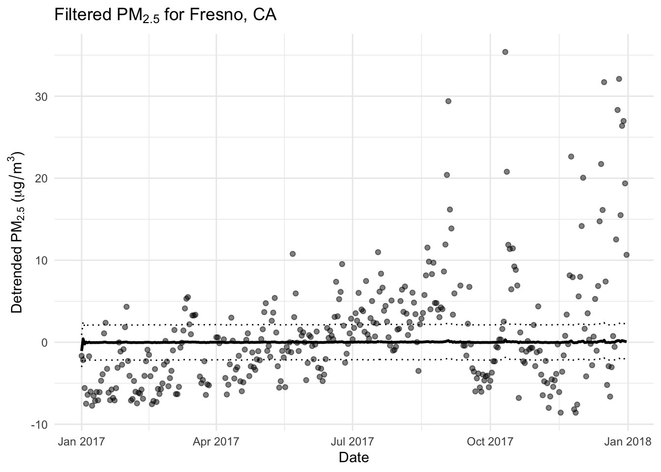
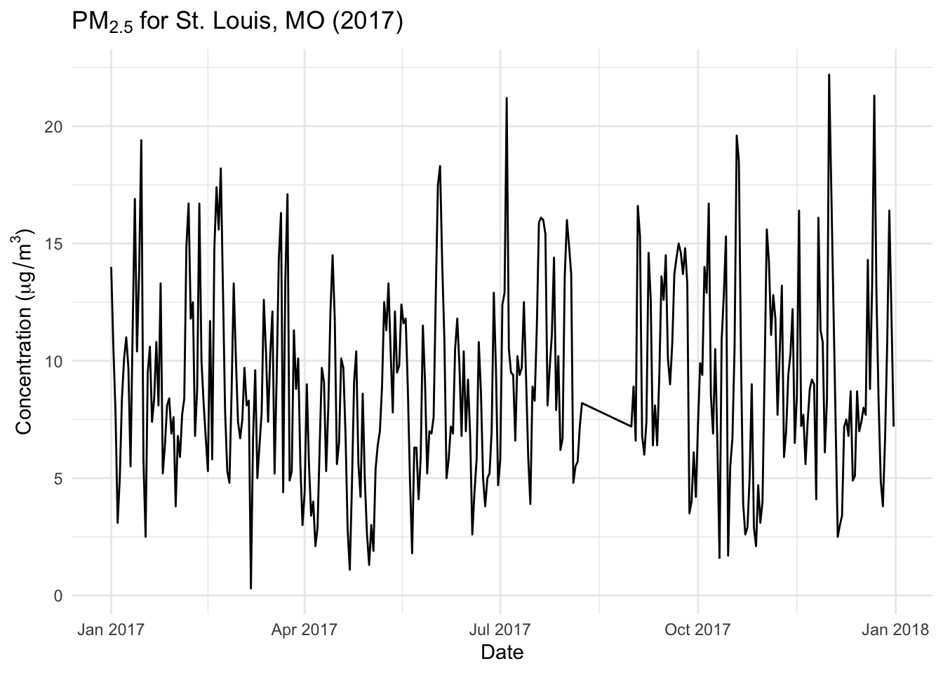
We will apply this model to the pollution data from St. Louis, Missouri shown previously.

First, let’s grab just the pollution series, convert to a tsibble and fill in the missing values with NAs.

   Min. 1st Qu.  Median    Mean 3rd Qu.    Max.    NA's 
  0.300   5.975   8.550   9.012  11.725  22.200      25 

     theta        tau        x00        P00          A      sigma 
 0.1483485  1.0000000 34.1221077  0.0000000  1.0000000  3.9401311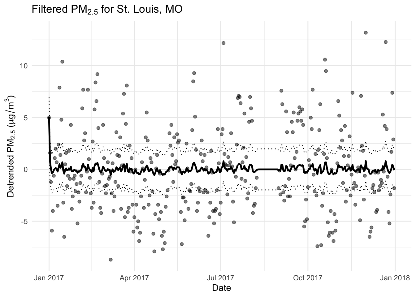 

   Min. 1st Qu.  Median    Mean 3rd Qu.    Max.    NA's 
-13.047  -5.269  -2.072   0.000   2.224  47.595      15 

     theta        tau        x00        P00          A      sigma 
-0.4098604  1.0000000  2.5825406  0.0000000  0.5000000  8.2580849